 KnowML
Sequence Modeling Pre-Transformer
Before any token could look directly at any other token, a whole generation of architectures squeezed the whole sequence through one running summary. The way that summary broke, mechanically, is the reason attention exists.
A recurrent network reads a sequence one element at a time. It keeps a single hidden-state vector as its "memory," updated at every step by the same shared weights. That reuse is exactly what kills it.
Backpropagating an error signal $t$ steps back multiplies it by the same Jacobian $t$ times, so the signal either vanishes toward zero or explodes. In practice it vanishes almost always, and long-range dependencies get forgotten.
LSTMs and GRUs patch this with gates that give the gradient a near-linear, additive path through time. Seq2seq chains two RNNs together for translation, but forces the entire input through one fixed-size vector: a second bottleneck. One sentence for an interview: RNNs forget because gradients decay multiplicatively over time, and the fixes either build a straighter path for the gradient (LSTM/GRU) or remove the sequential bottleneck entirely (attention).
01Intuition
A recurrent network reads like you do when you can't flip back a page.
Imagine reading a novel one word at a time. After every word you must compress everything you have read so far onto a single index card. A fixed number of slots, no matter how long the book gets.
You read the next word, glance at the card, update it, and throw away the exact wording of everything before it. By page 300 that card still has the same number of slots it had on page 1.
Early details survive only if they got re-written onto the card at every single page. Anything that stopped being relevant for a few dozen pages gets overwritten, and is effectively gone.
That index card is the RNN's hidden state. It's a fixed-size vector, and it's the network's only channel for carrying information from the past into the present.
Before RNNs, Markov chains and HMMs did not even pretend to keep a full running card. They explicitly assumed the next state depends only on the last one or two, and modeled language as a table of next-word probabilities conditioned on a short fixed window.
RNNs were the first attempt to make that window "as long as it needs to be." The summary became a learned, continuously-updated vector where a hard-coded lookup used to be.
Here is the catch, which explains the rest of this page. Writing to that card at every step is also how the network learns, via backpropagation. The further back an important word was, the more times its influence has to survive being multiplied through the update rule to reach the present. That repeated multiplication is where the story of LSTMs, GRUs, and eventually attention begins.
A recurrent network passes information through the same weight at every step, so a gradient sent back through many steps is multiplied by that weight many times.
Try it Multiply a gradient by the same weight twenty times
w = 0.5                        # a recurrent weight below 1
grad = 1.0
for t in range(1, 21):
    grad *= w                  # each step back multiplies the gradient
    if t in (1, 5, 10, 20):
        print(f"{t:>2} steps back: gradient x {grad:.7f}")

print(f"\nwith w = 1.5, after 20 steps: x {1.5 ** 20:,.0f}")0.5, the gradient is 0.5 after one step and about a millionth after twenty. Early inputs then have almost no influence on learning. With a weight of 1.5, the same twenty steps multiply it by 3,325 instead. Both directions break training, and that is the problem the rest of this page is about.02Timeline
Fixed-window n-gram models and Hidden Markov Models assumed the near future depends only on a small window of the recent past, so they could not use context from ten words back, let alone a hundred.
RNNs (1980s–90s, revived in the 2010s) carry a hidden state across timesteps, and LSTM (Hochreiter & Schmidhuber, 1997) and GRU add gates so that long-range memory works in practice.
Seq2seq (Sutskever et al., 2014) still squeezed the input into one vector, Bahdanau attention (2015) let the decoder look back at every encoder state, and in 2017 Vaswani et al. asked what happens if you delete the RNN and keep only the attention (page 08).
03Architecture: how the data flows
An RNN applies the same set of weights at every timestep. At step $t$ it takes two things: the current input $x_t$ and the previous hidden state $h_{t-1}$. Out comes a new hidden state $h_t$. Unrolling the network across a sequence means drawing that one cell repeated once per timestep, with the hidden state threaded through as the connecting wire.
Because $h_t$ strictly depends on $h_{t-1}$, you cannot compute step 500 before step 499 finishes. The recurrence is inherently sequential. That's the direct cause of the "RNNs can't parallelize across the sequence dimension" fact that shows up constantly in interviews. There's no way to compute all timesteps at once the way a Transformer's attention layer can, because each step's input literally depends on the previous step's output.
Bidirectional RNNs are a cheap, effective fix for one specific limitation. A plain left-to-right RNN's hidden state at position $t$ knows only about words before $t$, never after.
Where the whole sequence is available upfront, you can run a second RNN right-to-left over the same input and concatenate the two hidden states at each position. Now every position has context from both directions. That applies to tasks like:
- Tagging. Part-of-speech or named-entity labels, where the word after often disambiguates the word before.
- Classification. The whole sentence is in hand before you need a verdict.
- Encoding for translation. The source sentence is fully known; only the target is generated left to right.
This doesn't fix vanishing gradients. It fixes a blind spot. That's why encoders in seq2seq systems were very often bidirectional, while decoders never were. A decoder generates left to right and can't peek at words it hasn't produced yet.
04The equations
The vanilla RNN update, at every timestep:
- h_t the hidden state after processing $t$ elements. A fixed-size vector, and the network's entire memory of everything it has seen so far.
- W_h, W_x weight matrices shared across every timestep. The same $W_h$ multiplies the hidden state whether it's step 2 or step 200.
- x_t is the input at this timestep (e.g. a word embedding).
- tanh squashes the result to $(-1, 1)$, keeping the state bounded. Critically, its derivative is at most 1, and typically much less than 1 almost everywhere except near 0.
Why gradients vanish: the chain rule over time
To train the network, you need $\partial h_t / \partial h_0$ — how much the initial hidden state (and therefore anything that fed into it many steps ago) affects the state $t$ steps later. By the chain rule, this is a product of every intermediate Jacobian:
Each factor in that product involves the same matrix $W_h$, multiplied by a derivative of tanh bounded by 1. Multiply $t$ numbers that are each consistently a bit less than 1 and the product shrinks toward zero exponentially fast in $t$, which gives vanishing gradients.
The opposite can happen too. If the dominant eigenvalue of $W_h$ is greater than 1, the product grows exponentially instead. Those are exploding gradients, and they show up as loss suddenly spiking to NaN during training.
In practice vanishing is the far more common and more damaging failure. It doesn't crash training and silently leaves the model unable to learn dependencies more than roughly 10–20 steps apart.
This repeated-matrix-multiplication mechanism also appeared in 04 when initializing deep feedforward nets badly. An RNN unrolled over $t$ timesteps is, mathematically, a $t$-layer-deep network with tied weights at every layer.
LSTM: gates and the cell state
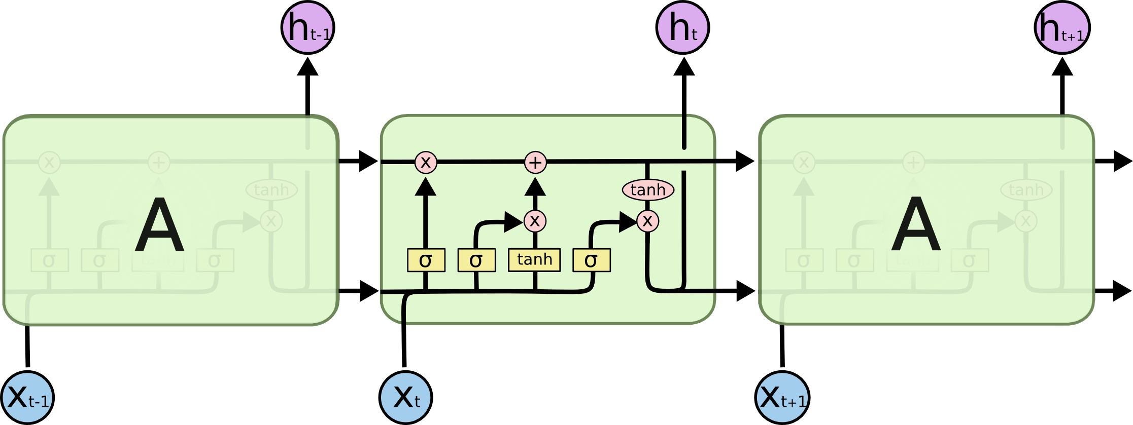
Hochreiter & Schmidhuber's 1997 fix keeps a second, separate piece of state: the cell state $C_t$. It is updated almost additively and is not repeatedly matrix-multiplied and squashed. Three gates control what happens to it, each a sigmoid-activated learned vector between 0 and 1:
- f_t forget gate. Decides what fraction of the old cell state to keep, per dimension. Near 1 means "remember this," near 0 means "erase this."
- i_t input gate. Decides how much of the new candidate information $\tilde{C}_t$ to write into the cell state.
- C̃_t candidate values. What the network could add to memory this step, before the input gate decides how much gets written.
- C_t the cell state update. A forget-gated copy of the old cell state plus an input-gated new candidate. The update is additive and elementwise, with a $+$ and no matrix multiply.
- o_t output gate. Decides how much of the squashed cell state gets exposed as the hidden state feeding the next layer and the next timestep.
GRU: the simpler cousin
The Gated Recurrent Unit (Cho et al., 2014) asks whether you need three separate gates and two separate states. It merges the cell state and hidden state into one. Forget and input collapse into a single update gate $z_t$, joined by a reset gate $r_t$ controlling how much past state is used when computing the candidate:
Fewer parameters, fewer matrix multiplies per step, and in practice roughly comparable performance to LSTM on most tasks. That's why GRUs became the default "I need an RNN and I want it cheaper" choice in the years between LSTM's dominance and attention's takeover.
The core idea is the same as LSTM's: $h_t$ is a convex combination of the old state and a new candidate, an additive blend with no repeated matrix multiplication.
05Why gating fixes vanishing gradients
Go back to the cell state update: $C_t = f_t \odot C_{t-1} + i_t \odot \tilde{C}_t$. Differentiate $C_t$ with respect to $C_{t-1}$, ignoring the comparatively minor dependence of the gates themselves on $C_{t-1}$, and you get $\partial C_t / \partial C_{t-1} \approx f_t$.
Just the forget gate, elementwise. Not a repeated multiplication by a fixed weight matrix $W_h$ squashed through tanh every single step.
So if the network learns to set $f_t \approx 1$ for a dimension carrying an important long-range signal, the gradient passes through that step almost unchanged. Chain that across many steps.
The path is still $t$ steps long, but each step is now close to an identity multiplication, where before it was lossy. The network can learn to keep the highway open, and a vanilla RNN has no mechanism to stop it closing.
This is the trick behind the residual connection in a ResNet or a Transformer block (see 04 and 08): give information an additive, near-identity shortcut that a gradient can flow through undiminished, so it never has to pass through a transformation at every step. The transformation becomes an optional adjustment on top and is no longer the only path.
LSTM's cell state is a gradient highway through time, in exactly the sense a residual stream is a gradient highway through depth. Same failure mode: repeated lossy transformations. Same fix: an additive path that bypasses them.
Gating doesn't make the vanishing gradient problem disappear entirely. With poor initialization, or extremely long sequences of thousands of steps, LSTMs still degrade. But it pushes the effective range of dependencies the network can learn from roughly 10-20 steps to several hundred. That was enough to make RNNs useful for translation, speech, and language modeling for most of the 2010s.
06RNN vs. LSTM vs. GRU vs. Transformer
| Vanilla RNN | LSTM | GRU | Transformer | |
|---|---|---|---|---|
| Parallelizable across sequence | No | No | No | Yes, fully |
| Max useful dependency range | ~10–20 steps | Several hundred steps | Several hundred steps | $O(1)$ path, any distance |
| Gate / gradient path | None — repeated $W_h$ · tanh' every step | 3 gates, additive cell state | 2 gates, additive hidden state | No recurrence — direct attention weight |
| Params per cell (roughly) | $1\times$ baseline | $\sim4\times$ (4 weight sets) | $\sim3\times$ (3 weight sets) | Different regime — scales with $d_{model}^2$ and depth, not sequence length |
| Inference cost per generated token | $O(1)$, tiny state | $O(1)$, tiny state | $O(1)$, tiny state | Grows with KV cache — see 08 |
That last row is worth sitting with. RNNs never lost the argument on inference efficiency. A recurrent model's memory is a fixed-size vector regardless of how long the conversation gets, while a Transformer's KV cache grows with every token generated.
RNNs lost on trainability and parallelism at scale. That tradeoff is exactly why state-space models (Mamba-style) resurfaced in the 2020s as a research direction. See the 2026 status note on page 08.
07Build this
This page claims a vanilla RNN gives up somewhere around 10 to 20 steps, and that gating stretches that to several hundred. Both of those are numbers you can measure yourself, on a laptop CPU.
Train a recurrent network on the remember-one-bit task. The first element of the sequence is 0 or 1. Then come $T$ steps of noise, and the model must output that first bit at the end. Guessing scores 50%, so there is exactly one thing to look at. Sweep $T$ and find where the model stops beating a coin.
- Write the vanilla RNN cell by hand from the update rule in section 04, plus one linear head on the final hidden state. Avoid
nn.RNN. - Generate the task on the fly. Train a fresh model for each gap length $T$ in 5, 10, 20, 40, 80, 160.
- Plot final accuracy against $T$. Mark the length where the curve drops to chance and stays there.
- Log the gradient norm at the first timestep, $\lVert \partial \mathcal{L} / \partial h_1 \rVert$, for every $T$. Plot it on a log axis beside the accuracy curve.
- Swap in an LSTM cell, also written by hand from the six equations in section 04. Rerun the identical sweep, extending it to longer $T$ until this one fails too.
- Now break the LSTM on purpose. Initialise the forget-gate bias to a large negative value, so $f_t$ starts near 0, and rerun the sweep.
Where this runs in production: seq2seq machine translation, pre-attention
Sutskever, Vinyals & Le's 2014 "Sequence to Sequence Learning with Neural Networks" set up the architecture that dominated neural machine translation until attention arrived. Two pieces:
- Encoder LSTM. Reads the source sentence and produces one final hidden state.
- Decoder LSTM. Initialized with that vector, it generates the target sentence one word at a time, feeding each generated word back in as the next input.
During training you don't feed the decoder its own predictions, which are possibly wrong early on. You feed it the true previous word from the training data. This is teacher forcing, and it makes training converge much faster and easier to parallelize across timesteps within a batch.
But it creates a mismatch: at inference time there's no ground truth to feed back in, so the model must consume its own predictions, mistakes included, which it never practiced doing. That mismatch is exposure bias. Small errors early in generation can compound, because the model is now in a distribution of inputs (its own imperfect outputs) it rarely saw during training.
Sentences got noticeably worse as they got longer, for exactly the reason you'd expect. Everything the decoder knows about the source has to fit through one fixed-size vector, and the pressure on that vector only grows with sentence length. That's the precise, named problem Bahdanau attention was built to solve, and the one page 08 picks up from here.
Where this runs in production: CTC in speech recognition
Speech recognition has a labeling problem seq2seq doesn't directly solve. An audio signal sampled into, say, 200 frames needs to map to a transcript of maybe 12 words. You don't know in advance which frames correspond to which letters. There's no frame-level alignment in the training data.
Connectionist Temporal Classification (CTC) solves this in two moves:
- Emit at every frame. The network outputs a probability distribution over characters, plus a special "blank" token, at every frame.
- Collapse many-to-one. A fixed rule (merge repeated characters, drop blanks) maps many different frame-level output sequences onto the same final transcript.
Training sums the probability over every alignment that collapses to the correct label, using dynamic programming. Per-frame labels are never required.
The key structural difference from seq2seq is alignment. CTC assumes monotonic alignment, where frame order matches output order and is never reordered, and produces one output per input frame that then gets collapsed. Seq2seq's encoder-decoder has no such constraint. It can freely reorder or vary output length relative to input length, which is necessary for translation where word order differs between languages, but more than speech recognition needs.
CTC-based and CTC-hybrid systems are still in production in real-time speech recognition today. The monotonic assumption holds there, and the lower latency of a single forward pass matters, with no separate decoder generating token by token.
08Interview questions
BeginnerWhat does an RNN's hidden state actually represent?
A fixed-size vector that's the network's entire summary of everything it has read so far. It's recomputed at every timestep from the previous hidden state and the current input using the same shared weights, which is what lets the network handle sequences of any length with a fixed number of parameters — and also what forces arbitrarily long histories through a fixed-size bottleneck.
BeginnerWhy can't RNNs parallelize across the sequence dimension?
Because $h_t$ is defined as a function of $h_{t-1}$ — you literally cannot compute the hidden state at step $t$ until you have the hidden state at step $t-1$. That sequential data dependency means processing a length-$n$ sequence takes $n$ sequential steps no matter how much parallel hardware you have, unlike a Transformer where every position's attention computation is independent and can run simultaneously.
IntermediateWalk me through exactly why vanilla RNN gradients vanish over long sequences.
$\partial h_t/\partial h_0$ is a product of $t$ Jacobians, each roughly $\text{diag}(\tanh') \cdot W_h$ — the same weight matrix and a tanh derivative bounded by 1, multiplied together $t$ times. If the typical factor is less than 1 (the common case), the product shrinks exponentially with $t$, so gradients from far-future errors barely reach far-past parameters — the network can't learn long-range dependencies, not because it doesn't need to, but because the learning signal never arrives intact. If the dominant eigenvalue of $W_h$ exceeds 1, you get the opposite failure — exploding gradients.
IntermediateWalk me through why LSTMs fix vanishing gradients.
LSTM keeps a separate cell state updated additively: $C_t = f_t \odot C_{t-1} + i_t \odot \tilde C_t$. Differentiating that with respect to $C_{t-1}$ gives approximately just the forget gate $f_t$, not a repeated multiplication by a fixed weight matrix squashed through tanh. If the network learns $f_t \approx 1$ for dimensions carrying important long-range information, the gradient passes through that step almost unchanged — an additive, near-identity path, the same mechanism as a residual connection, just through time instead of through depth.
IntermediateGRU vs. LSTM — when would you pick one over the other?
GRU merges the cell and hidden state into one and uses two gates instead of three, so it has fewer parameters and is cheaper per step. Empirically the two perform comparably on most tasks; GRU is the reasonable default when you want a lighter, faster-to-train recurrent model, LSTM when you have the compute budget and want the extra expressiveness of a separate, more protected cell state. In an interview, the important part is knowing they solve the same problem (multiplicative gradient decay) with the same core mechanism (an additive gated update) — the exact gate count is a secondary detail.
IntermediateWhat's the difference between teacher forcing and exposure bias?
Teacher forcing is a training-time choice: feed the decoder the ground-truth previous token instead of its own prediction, which speeds up and stabilizes training. Exposure bias is the consequence at inference time: the model never practiced conditioning on its own (possibly wrong) outputs, so at generation time small early mistakes push it into an input distribution it wasn't trained on, and errors can compound across the sequence.
DeepWhy does seq2seq degrade on long sentences, specifically, and how does attention fix it?
The decoder's only view of the entire source sentence is the encoder's final hidden state — one fixed-size vector, regardless of whether the source is 5 or 50 words. As sentence length grows, that vector has to compress proportionally more information into the same number of dimensions, and early words in the source are also the ones that had to survive the most sequential updates to even reach that final state — compounding the vanishing-gradient problem with a genuine information bottleneck. Attention removes the bottleneck by letting the decoder access every encoder hidden state directly at every decoding step, weighted by relevance, instead of relying on all of them being compressed into one vector — see 08 for the full mechanism.
DeepHow does CTC training work without frame-level alignment labels, and how is that different from seq2seq?
CTC outputs a distribution over the label vocabulary plus a blank token at every input frame, then defines a deterministic collapsing function (merge adjacent repeats, drop blanks) mapping many possible frame-level sequences to one label sequence. Training marginalizes — sums the probability — over every alignment that collapses to the correct label, computed efficiently with a forward-backward dynamic program, so no frame-level ground truth is ever needed, only the final label sequence. This requires monotonic, one-input-frame-to-one-output-slot alignment. Seq2seq has no such constraint — the decoder generates one token at a time conditioned on the whole encoded input (or, with attention, all encoder states) and can reorder or change length freely relative to the input, which is necessary for translation but is more flexibility than monotonic tasks like speech-to-text strictly require.
09Go deeper
●Now write it yourself
Reading the derivation and being able to produce it are different skills. These are Deep-ML problems that exercise what this page covers — each one is checked against real test cases, not multiple choice.
Matched to this page from Deep-ML's catalogue of 1,380 problems. More at deep-ml.com, and Where to practise covers the other platforms and what each one trains.