 KnowML
Generative Models
Discriminative models learn to tell classes apart. Generative models learn the whole data distribution, well enough to sample brand-new examples from it. This page follows that idea through VAEs, GANs, and the diffusion models running almost every image and video generator you've used.
A discriminative model learns $P(\text{label}\mid\text{data})$: a decision boundary. A generative model learns $P(\text{data})$ itself, well enough to draw new samples from it. VAEs and GANs were the two dominant ways to do this through the 2010s. Both work, and both have real, well-documented failure modes.
Diffusion models sidestep those failure modes by turning generation into something almost boringly simple: learn to reverse a slow, fixed process of adding noise, one small step at a time. One sentence for an interview: diffusion models don't learn to jump from noise to image in one shot. They learn to slightly improve a noisy image, over and over, which is a far easier thing to learn.
01Intuition
Generative vs. discriminative: what separates them
A classifier that tells cats from dogs only needs to find a boundary between the two classes. It never has to understand what makes a photo look like a plausible photo at all.
That is a discriminative model. It learns $P(\text{label}\mid\text{data})$, a function that maps inputs to outputs and nothing more.
A generative model is asked to do something much harder. It learns $P(\text{data})$ itself: the full distribution of "things that look like real photos". Well enough that you can draw a fresh sample from it and get something that was never in the training set but still looks like it belongs there.
Discriminative modeling asks for a boundary. Generative modeling asks you to understand the shape of the whole space well enough to invent a new point inside it.
Autoregressive generation — the idea from page 10, generalized
The simplest way to build a generative model is the one you already know from language models (10). Factor the joint distribution into a product of conditionals and predict one piece at a time: $P(x) = \prod_i P(x_i \mid x_{
For text that is next-token prediction. For images the same idea applies pixel by pixel, or more practically over discrete tokens produced by compressing the image first. Generate the top-left pixel, then the next one conditioned on it, and so on.
It works, and it gives an exact likelihood. Two things hold it back:
- Speed. Thousands of sequential steps for a single image.
- No revision. Once a pixel or token is generated, it is fixed. There is no notion of going back to improve an earlier guess.
That second limitation is a big part of why the field went looking for other factorizations of the generation process.
VAEs: compress, then regularize the compression
A plain autoencoder learns two things: an encoder that compresses an input into a low-dimensional latent code, and a decoder that reconstructs the input from that code. Train it well and reconstruction error goes to nearly zero.
But a plain autoencoder is not a generative model. Its latent space is just whatever shape minimizes reconstruction loss, with no constraint that nearby points decode to anything sensible. A random sample from it lands where the decoder has seen nothing like it, and you get garbage.
A Variational Autoencoder fixes exactly this, with two changes:
- The encoder no longer outputs a single latent code. It outputs the parameters of a distribution (a mean and a variance) over latent codes, and a sample is drawn from that distribution before being handed to the decoder.
- The loss adds a KL-divergence term that pulls every input's latent distribution toward a fixed, simple prior, usually a standard Gaussian.
The regularization forces the latent space to be smooth and densely packed around the origin, with no gaps.
So any point you sample from the prior decodes into something plausible. Not just points that came from encoding a real training image.
This is what separates an autoencoder that can only reconstruct memorized inputs from a VAE that can generate new ones.
Try it Same seed, same sample, and only one of them has a gradient
import torch
from torch.distributions import Normal
r = lambda t: [round(v, 3) for v in t.tolist()]

mu = torch.tensor([0.5, -1.0], requires_grad=True)
sd = torch.tensor([0.8, 0.3], requires_grad=True)
q = Normal(mu, sd)            # what the encoder emits for one input

torch.manual_seed(0)
z_bad = q.sample()            # the draw happens inside the graph
print("sample() ", r(z_bad), "grad_fn", z_bad.grad_fn)
try:
    z_bad.sum().backward()
except RuntimeError as e:
    print("backward:", str(e).split(" and")[0])

torch.manual_seed(0)
z_ok = q.rsample()            # the randomness is pushed out to eps
print("rsample()", r(z_ok), "grad_fn", type(z_ok.grad_fn).__name__)
z_ok.sum().backward()
print("dL/dmu   ", r(mu.grad), " dL/dsd", r(sd.grad))

torch.manual_seed(0)
eps = torch.randn(2)          # the same draw, written out by hand
print("by hand ", r(mu + sd * eps), " eps ", r(eps))sample() and rsample() both return [1.733, -1.088] — same seed, same eps — but the first arrives with grad_fn None and backward() flatly refuses it. The second carries an AddBackward0, because it was built as mu + sd * eps, which the last line reproduces by hand. Then look at dL/dsd: [1.541, -0.293], which is exactly the eps that was drawn. Moving the randomness outside turned it into a constant the gradient flows past, where it was an operation the gradient had to flow through. This is the reparameterization trick, and without it the encoder half of a VAE cannot be trained at all.GANs: two networks playing a game
A GAN trains two networks against each other:
- The generator maps random noise to a fake sample, trying to fool the other network.
- The discriminator looks at real and fake samples and tries to tell them apart.
Train both simultaneously and, in the ideal case, the generator gets pushed to produce samples indistinguishable from real data. No explicit density is ever modeled. The generator just learns to sample well.
GANs have two genuine, well-documented failure modes that were never fully solved in general, and they are not minor historical footnotes:
- Mode collapse. The generator discovers a handful of outputs that reliably fool the current discriminator and stops producing anything else. Diversity collapses even while individual samples look fine.
- Training instability. Two networks chase a moving target with no natural stopping criterion. The pair is prone to oscillation, and vulnerable to a discriminator that gets too good too fast and leaves the generator with a vanishing gradient signal.
Careful architectures and loss variants (Wasserstein GANs, spectral normalization, and others) reduced how often this happens. But "will this GAN converge nicely" was never something you could assume.
Derivation What the GAN loss is secretly minimising
The minimax objective looks like an arbitrary game somebody invented. It is not. Hold the discriminator at its optimum and the whole thing collapses into a recognisable distance between two distributions.
-
$$\begin{aligned} \min_G \max_D V(D, G) \;=\;\; & \mathbb{E}_{x \sim p_{\text{data}}}\!\left[\log D(x)\right] \\[2pt] +\;\; & \mathbb{E}_{z \sim p_z}\!\left[\log\big(1 - D(G(z))\big)\right] \end{aligned}$$The setup. The discriminator wants to output 1 on real data and 0 on fakes, so it maximises. The generator wants the opposite, so it minimises. Notice what is absent: no density is ever written down. $G$ only produces samples.
-
$$\begin{aligned} V(D, G) = \int_x \Big[\;\; & p_{\text{data}}(x) \log D(x) \\[2pt] +\;\; & p_g(x) \log\big(1 - D(x)\big) \Big]\, dx \end{aligned}$$Why this is legal: pushing $z$ through $G$ induces some distribution $p_g$ over samples, even though we cannot write it down. Re-expressing the second expectation over $p_g$ rather than $p_z$ puts both terms under a single integral in $x$. We never need a formula for $p_g$. We only need it to exist.
-
$$\begin{aligned} &\text{maximise} \quad f(y) = a \log y + b \log(1 - y) \\[2pt] &\text{where } \; a = p_{\text{data}}(x), \quad b = p_g(x) \end{aligned}$$Why we may optimise pointwise: $D$ is free to return whatever value it likes at each $x$, independently of every other $x$. An integral of independent terms is maximised by maximising each term separately. This step needs $D$ to range over all functions, and that is precisely where the theory quietly parts company with a finite network.
-
$$\begin{aligned} f'(y) &= \frac{a}{y} - \frac{b}{1-y} = 0 \\[4pt] \Longrightarrow \quad D^*(x) &= \frac{p_{\text{data}}(x)}{p_{\text{data}}(x) + p_g(x)} \end{aligned}$$Why: solve for the stationary point, then check $f''(y) = -a/y^2 - b/(1-y)^2 < 0$, so it is a maximum rather than a minimum. Read the answer aloud. The best possible discriminator reports the fraction of the density at $x$ that is real.
-
$$\begin{aligned} C(G) = V(D^*, G) \;=\;\; & \mathbb{E}_{p_{\text{data}}}\!\left[\log \frac{p_{\text{data}}}{p_{\text{data}} + p_g}\right] \\[2pt] +\;\; & \mathbb{E}_{p_g}\!\left[\log \frac{p_g}{p_{\text{data}} + p_g}\right] \end{aligned}$$Why: substitute $D^*$ back in. The second term works because $1 - D^*(x) = p_g/(p_{\text{data}} + p_g)$, which makes it a mirror image of the first. The generator now faces a fixed objective with no discriminator left in it.
-
$$C(G) = 2 \cdot D_{\mathrm{JS}}\!\left(p_{\text{data}} \,\|\, p_g\right) - \log 4$$Why: Jensen-Shannon divergence is $\tfrac{1}{2}D_{\mathrm{KL}}(P\|M) + \tfrac{1}{2}D_{\mathrm{KL}}(Q\|M)$ with $M = (P+Q)/2$. Each expectation above is one of those KL terms missing a factor of 2 inside its logarithm. Insert the 2 and compensate, and each term sheds a $\log 2$. Two of them give $-\log 4$.
-
$$\begin{aligned} \min_G C(G) = -\log 4 \quad &\text{iff} \quad p_g = p_{\text{data}} \\[2pt] &\text{at which } \; D^*(x) = \tfrac{1}{2} \end{aligned}$$Why: JSD is non-negative, and zero only when the two distributions match exactly. So the game has one global optimum, and at it the discriminator is reduced to a coin flip. It is not being fooled. It genuinely cannot tell.
Diffusion: learn to un-shred a photo, one small step at a time
The idea that made everything above easier to avoid: never ask a network to go straight from noise to a perfect image in one shot.
Take a real image and destroy it. Add a small amount of Gaussian noise, then a bit more, then a bit more, hundreds of times, until what is left is indistinguishable from pure static. This is the forward process, and nothing in it is learned: it is a fixed, known mathematical recipe.
Now train a network to do the single easiest version of the reverse job. Given a slightly-too-noisy image, predict what noise was added and remove a little of it. Not "generate the whole image". Just "make this one step less noisy".
Chain that one easy step backward, from pure noise all the way to $t{=}0$, and you have generated a new image. One small, well-defined denoising decision at a time.
That framing is what buys diffusion both of its advantages:
- More stable than a GAN. At every step there is a well-defined right answer (the noise that was added), so the network is doing ordinary supervised regression rather than chasing an adversary.
- Sharper than a plain VAE. A VAE asks one decoder to nail the entire reconstruction in a single forward pass, which encourages hedging toward a blurry average. Diffusion spreads the work across hundreds of small, low-stakes corrections, each of which the network can learn to do well.
02Timeline
VAEs (2013) trained stably but gave blurry samples, while GANs (2014) gave sharp samples but needed an unstable adversarial game between two networks.
DDPM (2020) learns to reverse a fixed noising process by regressing the noise, with no adversary, and latent diffusion (2022, Stable Diffusion) made it practical by working in a compressed latent space.
Diffusion became the default for image, video and audio generation, and by 2023–2024 Diffusion Transformers (DiT) increasingly replace the U-Net as the denoiser.
03Architecture: how the data flows
Two processes run in opposite directions over the same sequence of increasingly noisy images $x_0, x_1, \dots, x_T$:
- The forward process $q$ is fixed and requires no learning. It is just "add a bit of Gaussian noise, according to a known schedule".
- The reverse process $p_\theta$ is the one neural network in this whole picture. It is trained to undo one forward step at a time.
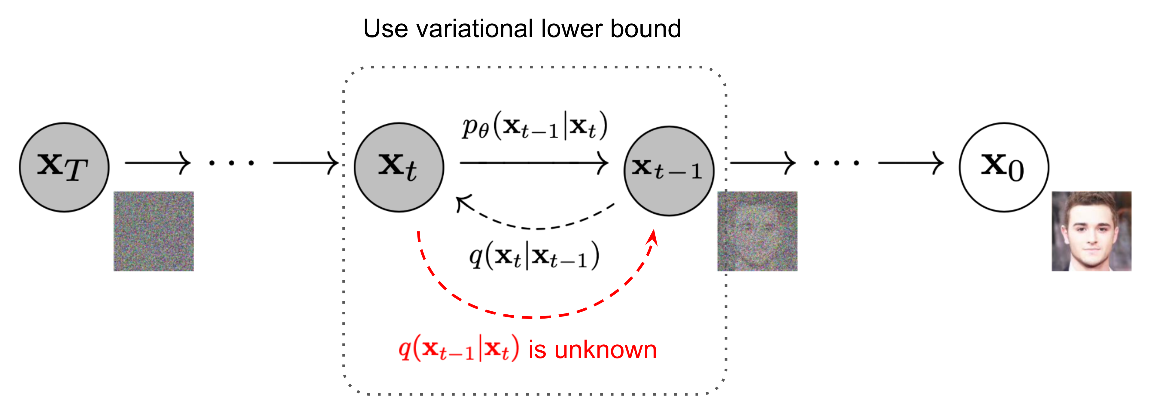
What does $\epsilon_\theta$ look like as a network? Two answers, a few years apart:
- U-Net, originally. A convolutional encoder-decoder with skip connections between matching resolutions, the same backbone family used in image segmentation. A natural fit, because input and output are both full images: a noisy image in, a predicted noise map out.
- Diffusion Transformer (DiT), in more recent large-scale systems. Chop the (usually latent-space) image into patches, treat them like tokens, and run ordinary transformer blocks. The same architecture from 08, applied to image patches instead of text tokens, with cross-attention or embedded conditioning bringing in the prompt at every block.
DiT tends to scale more predictably with more compute and data, the same lesson the field already learned from the original NLP transformers.
Conditioning gets folded in at every denoising step. It might be text, a pose skeleton, a depth map, or an edge map. Two common mechanisms: cross-attention (query from the image, key/value from the conditioning), or directly adding a conditioning embedding into the network.
ControlNet-style approaches take this further. Freeze a pretrained diffusion model entirely, then train a small parallel branch that reads an extra conditioning signal (edges, pose, depth) and injects its influence into the frozen network's intermediate activations. That gives precise structural control, exact pose and exact layout, without retraining or damaging the original model's learned knowledge.
04The equations
The forward process is designed so you can jump straight to any noise level $t$ in one step, without simulating all the steps before it: $x_t = \sqrt{\bar\alpha_t}\, x_0 + \sqrt{1-\bar\alpha_t}\, \epsilon$.
Here $\epsilon \sim \mathcal{N}(0, I)$ is fresh Gaussian noise, and $\bar\alpha_t$ is a known, fixed schedule value that decreases from near 1 (almost no noise) to near 0 (almost pure noise) as $t$ increases. That is the whole forward process, with no network involved and only algebra.
Try it Jump 400 noising steps in one multiply, and watch the signal go
import numpy as np
rng = np.random.default_rng(0)

T = 1000
betas = np.linspace(1e-4, 0.02, T)      # the DDPM linear schedule
abar = np.cumprod(1.0 - betas)          # alpha-bar_t, one per step
x0 = np.array([0.9, -0.7, 0.5, -0.3])   # a 4-pixel "image"

# The slow way: 400 real noising steps, on 20k copies at once.
x = np.repeat(x0[None], 20000, axis=0)
for t in range(400):
    z = rng.normal(size=x.shape)
    x = np.sqrt(1 - betas[t]) * x + np.sqrt(betas[t]) * z
print("x", tuple(x.shape))
print("400 steps:", np.round(x.mean(0), 3),
      "+/-", round(float(x.std(0).mean()), 3))

a = abar[399]                           # the same law, no loop at all
print("1 step:   ", np.round(np.sqrt(a) * x0, 3),
      "+/-", round(float(np.sqrt(1 - a)), 3))

for t in (0, 250, 500, 999):
    xt = np.sqrt(abar[t]) * x0 + np.sqrt(1 - abar[t]) * rng.normal(size=4)
    print(f"t={t:4d} sqrt(abar)={np.sqrt(abar[t]):.3f}",
"x_t=", np.round(xt, 2))[0.392 -0.307 0.223 -0.126] with spread 0.895; the closed form gets [0.398 -0.309 0.221 -0.133] and 0.897 from a single multiply and no loop. This is why training is affordable: each image gets one random $t$, never a trajectory. The other column worth reading is sqrt(abar). By t=500, the halfway point, only 0.279 of the original signal is left, and by t=999 it is 0.006 and x_t has no visible relation to x0. A linear $\beta$ schedule does most of its damage early, which is the complaint that later cosine schedules were built to fix.Before the diffusion loss, the VAE's. Diffusion inherits its whole argument, so it is worth having this one straight first.
Derivation Where the VAE loss comes from, line by line
We want to maximise $\log p(x)$. We cannot: it requires $p(x) = \int p(x \mid z)\, p(z)\, dz$, an integral over every possible latent. The way out is to stop computing it and start bounding it.
-
$$\log p(x) = \mathbb{E}_{q(z \mid x)}\!\left[\log p(x)\right]$$Why this is legal: there is no $z$ anywhere in $\log p(x)$. Taking an expectation over $z$ of something that does not depend on $z$ changes nothing. This looks like it does no work, but it is the move that lets us introduce $q$ at all.
-
$$= \mathbb{E}_{q}\!\left[\log \frac{p(x, z)}{p(z \mid x)}\right]$$Why: Bayes' rule, rearranged. Since $p(z \mid x) = p(x,z)/p(x)$, we can write $p(x) = p(x,z)/p(z \mid x)$.
-
$$= \mathbb{E}_{q}\!\left[\log \left( \frac{p(x, z)}{q(z \mid x)} \cdot \frac{q(z \mid x)}{p(z \mid x)} \right)\right]$$Why: multiply and divide by $q(z \mid x)$. This is the entire trick. It manufactures one term we can actually compute and one term we can bound.
-
$$= \underbrace{\mathbb{E}_{q}\!\left[\log \frac{p(x, z)}{q(z \mid x)}\right]}_{\text{ELBO}} \;+\; \underbrace{\mathbb{E}_{q}\!\left[\log \frac{q(z \mid x)}{p(z \mid x)}\right]}_{D_{\mathrm{KL}}(q \,\|\, p(z \mid x))}$$Why: the log of a product splits into a sum, and expectation is linear. The second term is exactly the definition of KL divergence between your encoder and the true posterior.
-
$$\log p(x) \;\geq\; \text{ELBO}$$Why: KL divergence is never negative. Drop a non-negative term from a sum and what remains is a lower bound. That inequality is the "LB" in ELBO.
-
$$\text{ELBO} = \underbrace{\mathbb{E}_{q}\!\left[\log p(x \mid z)\right]}_{\text{reconstruction}} \;-\; \underbrace{D_{\mathrm{KL}}\!\left(q(z \mid x) \,\|\, p(z)\right)}_{\text{regulariser}}$$Why: expand $p(x,z) = p(x \mid z)\,p(z)$ inside the ELBO, then group the two terms that depend only on $z$. Both pieces are now computable: the first by decoding a sample, the second in closed form for Gaussians.
Try it Turn the KL dial and watch the other half of the ELBO pay for it
import torch

x = torch.tensor(2.0)      # one data point; the decoder is the identity

def terms(mu, logsd):
    sd = logsd.exp()
    recon = (mu - x) ** 2 + sd ** 2          # E_q[(x - z)^2], exactly
    kl = 0.5 * (mu ** 2 + sd ** 2 - 1) - logsd
    return recon, kl

print(f"{'beta':>5}{'mu':>8}{'sigma':>8}{'recon':>8}{'KL':>8}")
for beta in [0.01, 0.1, 1.0, 4.0, 50.0]:
    p = torch.zeros(2, requires_grad=True)   # [mu, log sigma]
    opt = torch.optim.Adam([p], lr=0.02)
    for _ in range(4000):                    # this is all training does
        recon, kl = terms(p[0], p[1])
        opt.zero_grad()
        (recon + beta * kl).backward()       # the only knob is beta
        opt.step()
    recon, kl = terms(p[0], p[1])
    print(f"{beta:5.2f}{p[0]:8.3f}{p[1].exp():8.3f}"
f"{recon:8.3f}{kl:8.3f}")beta=0.01 reconstruction is 0.005 and the KL is 4.134; at beta=50 they have swapped places, 4.660 and 0.003. No setting buys both. The beta=50 row is posterior collapse in two numbers: mu=0.077, sigma=0.981 — the encoder has stopped encoding and just emits the prior $\mathcal{N}(0,1)$ whatever the input, which costs nothing on the KL term and is worth nothing to the decoder. And note that the honest VAE, beta=1, already drags $\mu$ to 1.333 for a point sitting at 2.0. That gap is where the blur comes from.Training the reverse process reduces, after the derivation settles, to a strikingly simple objective:
- x_0 a real training image, sampled from the dataset.
- t a timestep sampled uniformly at random from $1$ to $T$ — every training step picks a different, random noise level to train on.
- ε the actual Gaussian noise you drew and added to $x_0$ to construct $x_t$ via the formula above — this is the ground-truth label.
- x_t the resulting noisy image at that timestep — this is what the network sees as input, along with $t$ itself.
- ε_θ(x_t, t) the network's prediction: "given this noisy image and this timestep, what noise do I think was added?"
- ‖·‖² plain L2 distance between the true noise and the predicted noise — an ordinary regression loss, nothing adversarial or exotic about it.
Derivation How a variational bound collapses into that one MSE line
Diffusion is a VAE whose latents are the whole noising trajectory $x_1, \dots, x_T$, and whose encoder $q$ is fixed by hand rather than learned. So it inherits the bound above, and the work is in simplifying it.
-
$$\log p(x_0) \;\geq\; \mathbb{E}_q\!\left[\log \frac{p_\theta(x_{0:T})}{q(x_{1:T} \mid x_0)}\right]$$Why: identical to the ELBO step above. The only change is that the latent is now a sequence, not a single $z$.
-
$$\begin{aligned}\mathcal{L} = \mathbb{E}_q\Big[\;&\underbrace{D_{\mathrm{KL}}\big(q(x_T \mid x_0)\,\|\,p(x_T)\big)}_{\text{no parameters}} \\[2pt] &+ \sum_{t>1} D_{\mathrm{KL}}\big(q(x_{t-1} \mid x_t, x_0)\,\|\,p_\theta(x_{t-1} \mid x_t)\big) \\[2pt] &- \log p_\theta(x_0 \mid x_1)\Big]\end{aligned}$$Why: both the forward and reverse joints factor into per-step terms, so the bound regroups into one KL per timestep. The first term contains no learnable parameters at all: both sides are fixed. It is a constant you can ignore.
-
$$q(x_{t-1} \mid x_t, x_0) = \mathcal{N}\big(x_{t-1};\, \tilde\mu_t(x_t, x_0),\, \tilde\beta_t I\big)$$Why this step matters most: the reverse of a noising step is intractable on its own. Conditioned also on $x_0$ it becomes an ordinary Gaussian with a closed-form mean. That is the entire reason $x_0$ is carried through the derivation.
-
$$D_{\mathrm{KL}} = \frac{1}{2\sigma_t^2}\left\lVert \tilde\mu_t(x_t, x_0) - \mu_\theta(x_t, t) \right\rVert^2 + C$$Why: fix the reverse process to have the same variance as the forward posterior, and the KL between two Gaussians collapses to a scaled squared distance between their means. Every KL in the sum is now a regression target.
-
$$\left\lVert \tilde\mu_t - \mu_\theta \right\rVert^2 \;\longrightarrow\; w_t \left\lVert \epsilon - \epsilon_\theta(x_t, t) \right\rVert^2$$Why: $x_t$ is an invertible function of $(x_0, \epsilon)$. Substituting that relation into $\tilde\mu_t$ rewrites the mean-matching problem as a noise-matching problem. Same objective, different coordinates, and the noise coordinates turn out to be much easier to learn in.
-
$$\mathcal{L}_{\text{simple}} = \mathbb{E}_{x_0, t, \epsilon}\left[\left\lVert \epsilon - \epsilon_\theta(x_t, t) \right\rVert^2\right]$$Why — and this is the honest part: the weights $w_t$ are simply dropped. That is not a mathematical simplification. Ho et al. found the unweighted version trains better, so the objective everyone uses is deliberately not the tight variational bound.
Notice what's not in this loss: no discriminator, no generator fighting anything, no minimax. Pick a random image, pick a random timestep, add the corresponding amount of noise, ask the network to predict that noise, compute MSE, backpropagate. It's supervised regression with an unusually clever choice of label.
At sampling time you start from $x_T \sim \mathcal{N}(0, I)$, pure noise. Then repeatedly use $\epsilon_\theta(x_t, t)$ to estimate and subtract off a bit of noise, stepping from $x_T$ down to $x_{T-1}$, then $x_{T-2}$, and so on to $x_0$.
The original DDPM sampler does this stochastically, adding a little fresh noise back in at each step to match the forward process exactly. It needs on the order of hundreds to a thousand steps.
DDIM reformulates the reverse process as non-Markovian and deterministic. Same trained network, but a sampling procedure that can skip steps and still land close to a good sample. That cuts generation from hundreds of steps to a few dozen with the same weights, which is the difference between diffusion being usable in a real product and not.
05Why this architecture
Why diffusion trains more stably than a GAN. A GAN's loss is defined by two networks simultaneously trying to outmaneuver each other, so there is no fixed target: the "correct" gradient for the generator changes every time the discriminator updates, and nothing guarantees the pair converges rather than oscillates.
Diffusion training has none of that. At every step there is a single, fixed, correct answer (the noise that was added), so it is ordinary supervised regression. No adversary means no oscillation and no mode collapse in the GAN sense. It also means a loss curve that corresponds to the model getting better, which makes debugging and hyperparameter tuning tractable in a way GAN training famously isn't.
Why diffusion runs in latent space. Running the forward/reverse process directly on pixels means every one of those hundreds of denoising steps is a full forward pass of a large network over a full-resolution image. At 512×512×3 or larger, that is expensive to the point of being impractical on consumer hardware.
Latent diffusion first trains a VAE-style encoder/decoder pair that compresses images into a much smaller latent grid. Commonly an 8× spatial downsampling, so a 512×512 image becomes something like a 64×64 latent. The entire diffusion process then runs inside that compressed space: forward noising, reverse denoising, all of it. The final denoised latent is decoded back to pixels with the VAE decoder only once, at the very end.
It is the single change that took diffusion from a research curiosity requiring serious compute to something that runs on a single consumer GPU, which is exactly why it is called Stable Diffusion.
06Complexity, failure modes, and what breaks
| GAN | VAE | Diffusion | |
|---|---|---|---|
| Sample quality | Sharp, high-fidelity when it works | Often visibly blurrier | Sharp, currently state of the art |
| Training stability | Notoriously unstable — adversarial balance | Stable — single well-behaved loss | Stable — plain regression loss |
| Sampling speed | Fast — one forward pass | Fast — one forward pass | Slow — many iterative steps (DDIM/distillation narrow this) |
| Likelihood estimation | No explicit likelihood at all | Approximate — optimizes a lower bound (ELBO) | Approximate — also a (reweighted) variational bound |
What breaks
- Mode collapse (GAN). The generator finds a small set of outputs that reliably fool the current discriminator and stops exploring the rest of the data distribution. You get variety-starved samples: individually convincing, collectively failing to cover the real diversity of the training data. Mitigations (Wasserstein loss, minibatch discrimination, spectral normalization) reduce how often this happens. None eliminate it as a possibility.
- Blurry samples (VAE). A pixel-wise reconstruction loss, averaged over every plausible way an ambiguous region could look, is minimized by outputting something close to the average of those possibilities. That average looks blurry. Stronger decoders and adversarial or perceptual losses on top of the VAE objective help. But the core tension never fully disappears: KL regularization is needed for a samplable latent space, and it pulls against sharp reconstruction.
- Slow multi-step sampling (diffusion). The original DDPM sampler needs hundreds to a thousand sequential network evaluations per sample. Each one is a full forward pass, and they cannot be parallelized, because each step depends on the output of the last. DDIM is the direct first response: deterministic, skip steps, same weights. Further speedups come from distillation techniques that train a student model to match what the multi-step teacher would have produced in far fewer steps, sometimes down to single digits.
Two other model families deserve a mention, even though they get less production use today.
- Normalizing flows. Build a generative model out of a sequence of invertible transformations. That gives you an exact log-likelihood via the change-of-variables formula, a real advantage over the approximate bounds every other family here relies on. The cost: every layer has to be restricted to invertible, easy-to-Jacobian-determinant operations. That constrains architecture choices, and has kept flows from matching GAN or diffusion sample quality at scale.
- Energy-based models. Instead of directly defining how to sample, define a scalar "energy" function that should be low for realistic data and high for everything else. Generation means searching for low-energy points, typically via iterative gradient-based sampling such as Langevin dynamics. Conceptually elegant, and closely related to score-based views of diffusion. But training them (typically via contrastive divergence) and sampling from them efficiently is hard, which has limited their production use relative to diffusion.
Evaluating generative models
Unlike a classifier, there is no single clean accuracy number here. Two imperfect options:
- FID (Fréchet Inception Distance) compares the statistics of real and generated image features under a pretrained classifier network. It is the most commonly reported number in papers. It is also a proxy: sensitive to the reference dataset and the feature extractor used, and known to not always track what humans prefer.
- Human preference evaluation (pairwise comparisons, "which image do you prefer") is closer to what matters for a product. It is expensive, slow, and still noisy across raters.
Use both as proxies to triangulate with. Neither is ground truth: a model can win on FID and still look worse to people, or the reverse.
07Build this
Classifier-free guidance
This is the single most practically important diffusion concept if you are using these models, and it is simpler than it sounds.
During training, the conditioning signal (a text prompt's embedding, say) is randomly dropped and replaced with a fixed "empty" token some fraction of the time. A common choice is around 10%. So the exact same network learns to predict noise two ways:
- $\epsilon_\theta(x_t, t, c)$: the conditional prediction, given the prompt.
- $\epsilon_\theta(x_t, t, \varnothing)$: the unconditional prediction, ignoring the prompt entirely.
At sampling time, compute both predictions and extrapolate away from the unconditional one, toward the conditional one, by more than the conditional prediction alone would give you:
where $w$ is the guidance scale. Illustrative: at $w{=}1$ you get the plain conditional prediction, with no extrapolation.
Push $w$ higher and you exaggerate the direction the prompt is already pulling the prediction, which produces images that adhere to the prompt much more strongly. Values in roughly the 7–15 range are commonly used defaults in practice; Stable Diffusion's original default sat around 7.5.
Push it too far and you trade away diversity, and start seeing oversaturated colors and artifacts. Guidance scale is a real dial with a real quality/adherence tradeoff, and there is no free lunch.
Guidance is the dial. The reverse process is the thing being steered, and it is small enough to build from scratch in an afternoon.
Train a diffusion model on 2D points instead of images. The data is make_moons: two interleaved crescents. With two dimensions you can plot the entire distribution at every timestep, so the reverse process stops being a diagram and becomes something you watch happen, with no U-Net, no latent space and no GPU.
- Sample a few thousand points from
make_moonswith a little noise. Scatter-plot them. That plot is your ground truth for the rest of the project. - Write the forward process straight from section 04: a linear $\beta$ schedule over a few hundred timesteps, precomputed $\bar\alpha_t$, then $x_t = \sqrt{\bar\alpha_t}\,x_0 + \sqrt{1-\bar\alpha_t}\,\epsilon$. Plot the cloud at several values of $t$ and watch the crescents dissolve.
- Make $\epsilon_\theta$ a small MLP. Input is the 2D point plus a sinusoidal embedding of $t$; output is a 2-vector, the predicted noise. Train with the plain L2 loss from section 04.
- Sample. Draw $x_T$ from $\mathcal{N}(0, I)$, run the reverse loop down to $x_0$, and scatter-plot the whole cloud every twenty steps. Stack the frames into an animation or a grid.
- Now break it twice. Keep the trained weights and cut the reverse loop to a handful of steps. Then retrain with the timestep input removed from the network entirely.
Where this runs in production
Three distinct pretrained components, chained together, each doing one well-scoped job:
- Text encoder. A pretrained language model or CLIP-style text tower turns the prompt string into a conditioning embedding.
- Latent diffusion U-Net or DiT. Starts from random noise in latent space and runs the reverse denoising loop, typically a few dozen steps under DDIM-style sampling, with classifier-free guidance applied at every step to sharpen prompt adherence.
- VAE decoder. The final denoised latent passes through once, producing the actual pixel-space image.
Guidance is not a fourth model. It carries no weights of its own: it runs the same denoising network twice per step, once conditioned and once not, then extrapolates between the two predictions.
Video generation runs the same core machinery, but adds a new problem: temporal consistency. It is not enough for every individual frame to look right. Consecutive frames need to agree on where objects are, how they are moving, and what they look like. Otherwise you get flicker, and objects that subtly warp between frames.
There are two approaches. One extends the denoising network with temporal attention or convolution layers that let it look across nearby frames. The other diffuses over a whole short clip's latent representation jointly, instead of generating each frame's noise independently. Both treat time as another axis the network has to get right and not as an afterthought bolted onto single-image diffusion.
08Where you meet this in the wild
Generative modelling stopped being about pretty pictures somewhere around 2022. The interesting uses now are the ones where the thing being sampled is not an image at all.
The pattern to notice: diffusion works wherever you can define a sensible way to add noise and a network that can undo it. Pixels were just the first domain where that was easy. Atoms, weather states, and robot trajectories turned out to work too.
- You need plausible new samples and no label: data augmentation, simulation, design search.
- The answer is one-to-many: many valid images fit a prompt, and many valid weather trajectories fit today's readings. A regressor forced to pick one will average them into mush.
- You need calibrated uncertainty and can get it by sampling repeatedly, rather than from a single confidence score.
- You want a learned latent space to work in, and generation is a side effect you may never use.
- You only need a decision boundary. A discriminative classifier will be smaller, faster and easier to evaluate.
- You need exact likelihoods. Diffusion and GANs do not give them cleanly, while normalizing flows do at a cost in expressiveness.
- Latency is tight and quality is negotiable. Iterative denoising is many forward passes; a one-shot model may be the better trade.
- You cannot define what "realistic" means for your data well enough to evaluate it. If you cannot tell a good sample from a bad one, you cannot train or ship this.
09Going deeper: the decisions that change your output
Everything above explains why diffusion works. This section is about the handful of choices that decide what you get out of it.
Inside Stable Diffusion, at inference
The pipeline above listed three components, but it did not say what each one costs you at generation time, and the distribution is lopsided.
- The text encoder runs once and is cheap enough to ignore.
- The denoising network runs once per step, and twice per step when guidance is on, so it is the entire compute budget.
- The VAE decoder runs once, at the end. Also cheap next to the loop.
So a 30-step generation with classifier-free guidance is 60 forward passes of a large network. Everything else rounds to zero.
The compression is 8× in each spatial dimension: a 512×512 image becomes a 64×64 latent.
Eight times in each direction means 64× fewer spatial positions to process. Every one of those 60 forward passes gets 64× cheaper.
That multiplier is the difference between a model that runs on a consumer GPU and one that does not.
The knobs, roughly in order of how much they move the result:
- Step count. Cost is linear in it. How low you can go depends entirely on the sampler.
- Guidance scale. Prompt adherence traded against diversity, covered above.
- Sampler. Changes the step floor by an order of magnitude, and costs nothing to swap.
- Resolution. Cost is quadratic in it, and quality also tends to degrade well away from the resolution the model was trained at.
Samplers: same weights, different arithmetic
A sampler is the rule for stepping from $x_t$ to $x_{t-1}$, and it is not part of the trained model at all. Swap it whenever you like.
| Sampler | Typical steps | Deterministic | Needs training |
|---|---|---|---|
| DDPM (ancestral) | Hundreds to ~1000 | No, injects fresh noise each step | No |
| DDIM | A few dozen | Yes | No |
| DPM-Solver | 10 to 20 | Yes | No |
| Distilled (e.g. LCM) | 1 to 4 | Yes | Yes, a distillation run |
DPM-Solver treats the reverse process as an ODE and applies a higher-order numerical solver to it. Same network, same weights, better integration. Its authors report high-quality samples in 10 to 20 network evaluations, a 4 to 16× speedup over previous training-free samplers.
DDPM, DDIM and DPM-Solver are not different models. They are different ways of numerically integrating the same learned reverse process.
You can download one checkpoint and get any of them, which is why sampler choice is the cheapest large speedup available to you.
The fourth row is different in kind. Getting below roughly ten steps means changing the weights.
Adaptation without retraining
Almost nobody trains one of these from scratch, so practical work is nearly all adaptation of a checkpoint someone else paid for. Five techniques cover most of what people do, and they differ mainly in how much of the model they are willing to disturb.
- LoRA. Freeze the base weights and learn a small low-rank update beside them. Proposed for language models, it transfers directly to diffusion. The files are small enough to swap and stack freely.
- DreamBooth. Fine-tune the model on a handful of images of one subject, bound to a rare identifier token. Strong subject fidelity. Also the heaviest option, and the most prone to overfitting a small reference set.
- Textual inversion. Keep the model entirely frozen and learn one new embedding vector for one new token. The smallest possible intervention, and correspondingly limited in what it can express.
- ControlNet. Clone the encoder and train the copy on a spatial conditioning signal: edges, depth, pose, segmentation. It controls composition, with content left to the prompt.
- IP-Adapter. Add a separate cross-attention path for image features, so an image can act as a prompt alongside the text. Roughly 22M parameters, and it composes with the others.
ControlNet has a detail worth stealing for your own work. The trained copy reconnects to the frozen base through zero-initialised convolutions. At the start of training those layers output nothing, so the branch is a no-op and cannot damage a working model. It grows its influence from zero as training proceeds.
Where GANs still win
Not many places, but the ones that remain are real and worth being precise about.
A GAN generator produces its output in one forward pass. Diffusion needs several at absolute minimum, usually dozens. When the latency budget is small and fixed, that gap decides the architecture on its own.
- Neural vocoding. HiFi-GAN emits a waveform in a single pass. A voice agent replying in real time cannot afford a denoising loop. See 13.
- Super-resolution and restoration. Real-ESRGAN-style models are still widely deployed for upscaling, where one pass is enough.
Notice what those share: the output is tightly constrained by the input, so the one-to-many problem that drives mode collapse is much smaller to begin with. Add a hard latency budget and the trade tips toward the GAN.
Few-step generation
Better samplers took diffusion from a thousand steps down to roughly ten, which is where training-free cleverness runs out. Going lower means changing the weights as well as integrating them more carefully.
Consistency models are trained so that every point along a trajectory maps directly to that trajectory's endpoint. If that property holds, you can jump straight to the answer instead of walking to it.
Latent consistency models apply the idea to an existing latent diffusion model by distilling it. The authors report 2 to 4 step generation at 768×768, distilled in roughly 32 A100-hours.
The trade is consistent across the whole family. You give up some quality and some diversity, you gain a large cut in latency, and you pay a distillation run up front.
Evaluation is the bottleneck
The failure-modes section introduced FID and human preference. Both are weaker than their ubiquity suggests.
The Rethinking FID analysis lays out the specific problems:
- Inception features were trained for classification. They represent the content of modern text-to-image output poorly.
- FID compares only the first two moments, which assumes the feature distributions are Gaussian, and typically they are not.
- Sample complexity is poor, so the number you get shifts with how many samples you scored.
- It can contradict human raters, and does not reliably track gradual improvement in a model.
That paper proposes CMMD instead, pairing CLIP embeddings with a maximum mean discrepancy distance.
Generative quality is easy to see and hard to measure, and no automated metric settles the question today.
10Interview questions
BeginnerWhat's the difference between a generative and a discriminative model?
A discriminative model learns $P(\text{label}\mid\text{data})$ — it only needs a boundary that separates classes, and never has to represent what makes data plausible in the first place. A generative model learns $P(\text{data})$ itself, well enough to sample brand-new, never-seen examples from that distribution.
BeginnerWhy isn't a plain autoencoder a generative model, but a VAE is?
A plain autoencoder's latent space is shaped only by reconstruction loss. Nothing guarantees that a random point in it decodes to anything sensible, so you cannot sample from it. A VAE adds a KL-divergence term that pulls every input's latent distribution toward a fixed prior, usually a standard Gaussian. That forces the space to be smooth and densely packed, with no gaps, so any point drawn from the prior decodes to a plausible output rather than a memorized reconstruction.
IntermediateWhy do diffusion models train more stably than GANs?
GAN training is an adversarial minimax game between two networks with no fixed target. The "correct" gradient for the generator keeps changing as the discriminator updates, and nothing guarantees convergence rather than oscillation or collapse. Diffusion training has one fixed correct answer at every step, the noise actually added, so it reduces to ordinary supervised regression with an L2 loss. There is no adversary to oscillate against, and the loss curve tracks improvement.
IntermediateWhat does classifier-free guidance actually do at sampling time?
The model was trained to predict noise both with the conditioning (e.g. a prompt) and without it (conditioning replaced by an empty token). At sampling time you compute both predictions and extrapolate away from the unconditional prediction toward the conditional one, scaled by a guidance weight $w>1$. This exaggerates the direction the prompt is already pulling the model, producing much stronger prompt adherence at the cost of some sample diversity, and can introduce artifacts if pushed too high.
IntermediateWhy does Stable Diffusion run in latent space instead of pixel space?
Diffusion needs many sequential network evaluations per sample. Running that directly on full-resolution pixels makes every one of those steps a full forward pass over a large image, which is expensive enough to be impractical on consumer hardware. Latent diffusion compresses images into a much smaller latent grid with a pretrained VAE encoder first, runs the entire noising/denoising process there, and decodes back to pixels only once at the end — the compute savings are what make diffusion tractable outside a datacenter.
DeepWalk me through the DDPM training objective — what is the network actually predicting, and why does that make it easy to train?
Sample a real image $x_0$, a random timestep $t$, and random Gaussian noise $\epsilon$. Construct the noisy image directly via $x_t = \sqrt{\bar\alpha_t}\,x_0 + \sqrt{1-\bar\alpha_t}\,\epsilon$ — no simulation needed. Feed $x_t$ and $t$ into the network and have it predict $\epsilon$; train with L2 loss between the true and predicted noise. It's easy to train because it's plain supervised regression with a well-defined, always-available label — you never need an adversary, a search procedure, or an intractable likelihood; you just need to be able to add noise and subtract it back off.
DeepWhat's mode collapse, and why is it still a genuinely hard, unsolved problem for GANs?
Mode collapse is when the generator converges on a small set of outputs that reliably fool the current discriminator and stops exploring the rest of the real data distribution — high-quality individual samples, low overall diversity. It's hard because the generator's objective only ever asks "can I fool the discriminator right now," with no explicit term rewarding coverage of the full data distribution — so a narrow, reliable strategy is a perfectly valid local optimum of the adversarial game. Architectural and loss-level mitigations reduce how often it happens in practice, but none of them change the underlying game-theoretic incentive that makes it possible in the first place.
11Go deeper
●Now write it yourself
Reading the derivation and being able to produce it are different skills. These are Deep-ML problems that exercise what this page covers — each one is checked against real test cases, not multiple choice.
Matched to this page from Deep-ML's catalogue of 1,380 problems. More at deep-ml.com, and Where to practise covers the other platforms and what each one trains.
Other techniques for this problem
A scoped slice of the full Technique Map — every technique this page covers, grouped by what it solves.