 KnowML
Attention & Transformers
The mechanism that let every token look directly at every other token, no matter how far apart. The single most interview-relevant idea in modern AI.
Attention computes, for every token, a weighted average of every other token's representation. The weights come from how relevant those tokens are to each other, and "relevant" is learned and is not hand-coded, which means recurrence can be dropped entirely.
Stack blocks of attention + a feed-forward layer with residual connections and normalization, and you get the Transformer: the architecture behind BERT, GPT, ViT, Whisper, and almost everything trained since 2018. One sentence for an interview: attention is a soft, differentiable, content-based lookup.
01Intuition
Attention is a soft dictionary lookup.
A Python dictionary matches one key exactly. d["cat"] hands back a single value and ignores everything else it holds.
Attention asks a fuzzier question. Not "which key matches?" but "how similar is my query to every key?" It then returns a blend of all the values, weighted by that similarity. Three steps:
- Score. Compare the query against every key. One similarity number per key.
- Normalize. Push those scores through a softmax so they sum to one.
- Blend. Take the weighted average of every value, using those weights.
Nothing is discarded, and every token contributes by a different amount.
"The animal didn't cross the street because it was too tired."
What does it refer to? On its own, the word is ambiguous. The animal, or the street.
Self-attention lets the representation of it act as a query and compare itself against every other word in the sentence. Animal scores far higher than street, because tiredness is a property of animals. So the output vector for "it" becomes mostly "it", blended heavily with "animal".
The ambiguity is resolved inside the representation itself, before any downstream layer ever sees it.
Here is the same idea in numbers. Three words each carry a two-number key that says how animal-like or object-like the word is. The word it sends out a query asking for something animal-like. The vectors are hand-picked to make the point; a trained model learns them.
Try it Attention on three words, with numbers you can check by hand
import numpy as np

words = ["cat", "mat", "it"]
K = np.array([[1.0, 0.0],        # "cat": an animal
              [0.0, 1.0],        # "mat": an object
              [0.5, 0.5]])       # "it": not sure yet
V = K.copy()                     # here each value is just its key
q = np.array([2.0, 0.5])         # what "it" is looking for: animal-like

scores = K @ q / np.sqrt(2)      # how well each word matches the query
w = np.exp(scores) / np.exp(scores).sum()   # softmax: weights sum to 1
out = w @ V                      # a weighted average of the values

for word, s, weight in zip(words, scores, w):
    print(f"{word:>4}: score {s:5.2f}  weight {weight:5.2f}")
print("new vector for 'it':", np.round(out, 2))it scores 1.41 against cat, 0.35 against mat and 0.88 against itself. The softmax turns those into weights of 0.52, 0.18 and 0.30, which sum to 1. The new vector for it is [0.67 0.33]: a weighted average of the three values, tilted toward the animal direction because cat got the biggest weight. Every word contributed, just by different amounts.That example is Jay Alammar's, from The Illustrated Transformer. Worth twenty minutes if diagrams land faster for you than equations.
Every self-attention layer does this for every token against every other token, all at once. Queries, keys, values, multiple heads and the $\sqrt{d_k}$ scaling are machinery that makes this one idea learnable and numerically well-behaved.
02Timeline
Seq2seq (2014) squeezed an entire input sentence into one fixed-size vector, so long sequences degraded badly.
Bahdanau attention (2015) let the decoder look back at every encoder state, and Vaswani et al., "Attention Is All You Need" (2017), dropped the recurrence and kept only attention plus position information.
BERT and GPT (2018) built on the encoder and decoder stacks, ViT (2020) showed the same block works on image patches, and by 2023 the Transformer was the default for text, vision, audio and increasingly robotics.
03Architecture: how the data flows
Every token's embedding is linearly projected three different ways: into a Query, a Key, and a Value vector. Three learned lenses on the same token.
- Query. "What am I looking for?"
- Key. "Here's what I contain."
- Value. "Here's what I'll give you if you attend to me."
Now wrap that in a block: a residual connection, a normalization layer, and a position-wise feed-forward network. Repeat that 12–96+ times and you have a Transformer stack:
That block, stacked, is the whole architecture. Here is how the original paper drew the full encoder-decoder picture: an encoder stack on the left, feeding a decoder stack on the right through cross-attention.
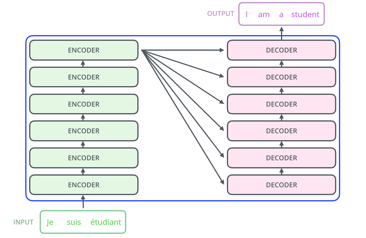
Shapes, concretely:
- Input token ids:
(batch, seq_len) - After the embedding table:
(batch, seq_len, d_model) - After a decoder-only LM head:
(batch, seq_len, vocab_size)logits, one distribution per position predicting the next token
Every attention and feed-forward layer preserves that middle shape. Attention mixes information across the seq_len axis but never changes it. Only the final LM head projects d_model → vocab_size.
Encoder and decoder stacks differ in exactly one line.
- Encoder (used in BERT). It is bidirectional, so every position sees the whole input at once.
- Decoder (used in GPT). It is causal, so each position sees only itself and earlier positions.
The decoder gets there by masking out future positions before the softmax, setting their scores to $-\infty$. Same mechanism, one masking triangle.
Try it Run scaled dot-product attention by hand, mask and all
import numpy as np
rng = np.random.default_rng(0)

T, d_k = 4, 8                    # 4 tokens, 8-dim queries and keys
Q = rng.normal(size=(T, d_k))
K = rng.normal(size=(T, d_k))
V = rng.normal(size=(T, 3))      # values need not share d_k

scores = Q @ K.T / np.sqrt(d_k)  # (T, T): everyone against everyone
future = np.triu(np.ones((T, T), dtype=bool), k=1)
scores[future] = -np.inf         # token t may not read past t

m = scores.max(axis=1, keepdims=True)
W = np.exp(scores - m)
W /= W.sum(axis=1, keepdims=True)     # softmax, one row at a time
Z = W @ V

print("Q", Q.shape, "K.T", K.T.shape, "scores", scores.shape)
print("W", W.shape, "V", V.shape, "Z", Z.shape, "\n")
print(np.round(scores, 2), "\n")
print(np.round(W, 3))
print("row sums:", W.sum(axis=1))
print("Z[0] is exactly V[0]:", np.allclose(Z[0], V[0]))W sums to exactly 1., including the first one. The mask sets the strict upper triangle to -inf, and exp(-inf) is 0, so row 0 has nowhere to look but itself — its weight is forced to 1.000 and the output Z[0] comes back as literally V[0]. The first token of a causal model gets no context at all, in every layer, forever. Row 3 is the only unconstrained one: 0.102 / 0.031 / 0.684 / 0.183, dominated by token 2 because 1.4 was its largest score. Notice too that scores is (4, 4) while V is (4, 3) — the attention matrix is square in sequence length and knows nothing about how wide the values are.04The equations
- Q, K, V matrices of shape
(seq_len, d_k)— every row is one token's query/key/value vector, produced by three separate learned linear layers on the input embeddings. - QKᵀ a
(seq_len, seq_len)matrix of raw similarity scores — every token compared against every other token via dot product. - √d_k scaling factor: without it, dot products of high-dimensional vectors grow large in magnitude, which pushes softmax into a region with near-zero gradients almost everywhere except one spike. Dividing by $\sqrt{d_k}$ keeps the variance of the scores roughly constant regardless of dimension, so training stays stable.
- softmax applied row-wise, turning each token's raw scores into a probability distribution over all tokens (including itself) that sums to 1.
- · V the weighted sum — multiplying those probabilities back into the value vectors gives, for each token, a blend of everyone else's information, proportioned by relevance.
Derivation Why $\sqrt{d_k}$, and not $d_k$ or any other constant
"Keeps the variance stable" is the usual hand-wave. It is a three-line calculation, and doing it tells you exactly why the exponent is one half. Follow the original paper and assume the components of $q$ and $k$ are independent, with mean 0 and variance 1. That assumption is what the whole argument rests on.
-
$$q \cdot k = \sum_{i=1}^{d_k} q_i k_i$$Setting up: the raw score for one query against one key is a sum of $d_k$ products. The question is how that sum behaves as $d_k$ grows.
-
$$\mathbb{E}[q_i k_i] = \mathbb{E}[q_i]\,\mathbb{E}[k_i] = 0$$Why the factorisation is legal: independence lets the expectation of a product split into a product of expectations. Both are zero by assumption, so every term is mean-zero and the whole score is centred at 0. The score does not drift as dimension grows. Only its spread does.
-
$$\operatorname{Var}(q_i k_i) = \mathbb{E}[q_i^2 k_i^2] - 0^2 = \mathbb{E}[q_i^2]\,\mathbb{E}[k_i^2] = 1 \cdot 1 = 1$$Why $\mathbb{E}[q_i^2] = 1$: variance is $\mathbb{E}[q_i^2] - \mathbb{E}[q_i]^2$, and the mean is zero, so the second moment equals the variance. That is the small step that makes this collapse so cleanly, and it only works because the components are centred.
-
$$\operatorname{Var}(q \cdot k) = \sum_{i=1}^{d_k} \operatorname{Var}(q_i k_i) = d_k$$Why the variances simply add: variance of a sum equals the sum of variances only when the terms are uncorrelated, which independence across $i$ gives us. Drop that assumption and this line fails. So the score's standard deviation is $\sqrt{d_k}$: it grows with the square root of head dimension, not with the dimension itself.
-
$$\operatorname{Var}\!\left(\frac{q \cdot k}{\sqrt{d_k}}\right) = \frac{d_k}{d_k} = 1$$Why this exact constant: dividing a random variable by $c$ divides its variance by $c^2$. To cancel a variance of $d_k$ you need $c^2 = d_k$, so $c = \sqrt{d_k}$. Dividing by $d_k$ would over-correct and crush the scores toward zero; dividing by anything else leaves a dimension-dependent scale. There is exactly one right answer.
Try it Watch the variance grow with d_k, and the softmax collapse
import numpy as np
rng = np.random.default_rng(0)

def dots(d_k, n=200_000):        # n independent q.k scores
    q = rng.normal(size=(n, d_k))
    k = rng.normal(size=(n, d_k))
    return (q * k).sum(1)

for d_k in (8, 64, 512):
    s = dots(d_k)
    print(f"d_k={d_k:4d}  var(q.k)={s.var():7.1f}"
          f"   var after /sqrt(d_k)={s.var()/d_k:.2f}")

def softmax(x):
    e = np.exp(x - x.max())
    return e / e.sum()

d_k = 512                        # one query against six keys
s = rng.normal(size=(6, d_k)) @ rng.normal(size=d_k)
p_raw, p_sc = softmax(s), softmax(s / np.sqrt(d_k))
print("\nraw scores:      ", np.round(s, 1))
print("unscaled softmax:", np.round(p_raw, 4))
print("scaled softmax:  ", np.round(p_sc, 4))
print(f"smallest weight: {p_raw.min():.1e} unscaled,"
      f" {p_sc.min():.1e} scaled")
var(q.k) comes out 8.0, 63.8, 510.9 — it is $d_k$. Dividing by $\sqrt{d_k}$ pins it at 1.00 in all three cases, which is the derivation above in one line of output. The second half shows why anyone should care. At $d_k=512$ the raw scores span -70.6 to 25.6, and softmax turns that into a weight of 1.6e-42 on the weakest key. The gradient flowing back through that entry is not small, it is gone. Scaled, the same six scores give 0.0056 through 0.3959: still a clear preference, still differentiable everywhere.Multi-head attention
Running one attention function gives the model exactly one notion of "relevance." In practice you want several. One head might learn to track subject-verb agreement, another coreference, another local syntax. Multi-head attention runs $h$ independent, smaller attention operations in parallel and concatenates the results:
If $d_{model}=512$ and $h=8$, each head works in $d_k = 64$ dimensions. The total compute is the same as one 512-dim head, and it buys 8 independent subspaces to specialize in, where a single head has to average everything together.
Try it Split one tensor into heads and confirm nothing was computed
import torch
torch.manual_seed(0)

T, d_model, H = 5, 12, 3         # 5 tokens, 3 heads of width 4
d_h = d_model // H
x = torch.randn(T, d_model)      # one projection's output, e.g. Q

heads = x.view(T, H, d_h).transpose(0, 1)   # (H, T, d_h)
print("x", tuple(x.shape), "-> heads", tuple(heads.shape))

# No arithmetic happened: the heads share x's memory.
print("same storage:", heads.data_ptr() == x.data_ptr())
print("head 1, token 0:", [round(v, 3) for v in heads[1, 0].tolist()])
print("x[0, 4:8]      :", [round(v, 3) for v in x[0, 4:8].tolist()])

# Each head gets its own (T, T) attention map, for the same FLOPs.
A = torch.softmax(heads @ heads.transpose(-2, -1) / d_h**0.5, -1)
print("attention maps:", tuple(A.shape))

back = heads.transpose(0, 1).reshape(T, d_model)   # the Concat step
assert torch.equal(back, x)
print("concat recovers x bit-for-bit:", torch.equal(back, x))
same storage: True is the key line. Splitting (5, 12) into three heads of width 4 is a view and a transpose — the split itself runs no arithmetic at all, and heads[1, 0] prints 0.849, 0.692, -0.316, -2.115 because those are the very same bytes as x[0, 4:8]. What the reshape buys is (3, 5, 5): three independent attention maps where one head would have given you one. The $\text{Concat}$ in the equation above is that reshape run backwards, and torch.equal(back, x) is True — bit-for-bit, not approximately. Multi-head costs no more, because it spends the same $d_{model}$ on more opinions.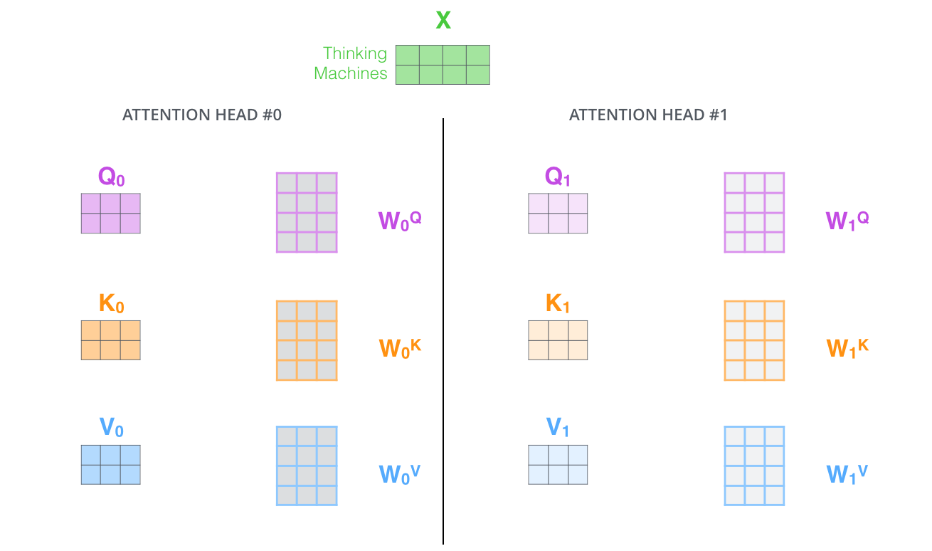
Positional information
Attention itself is permutation-invariant. Shuffle the input tokens and you get the same set of outputs, shuffled the same way, so the layer has no sense of order. Order has to be injected, and there are two standard ways to do it:
- Sinusoidal (original paper). Fixed position vectors added to the input embeddings, one frequency per dimension.
- RoPE, Rotary Position Embedding (modern default). Rotate each query/key vector by an angle proportional to its position.
RoPE's payoff is subtle but large. The dot product between a query at position $m$ and a key at position $n$ ends up depending on the relative distance $m-n$ and not on the absolute positions. This relative-distance property makes RoPE extrapolate more gracefully to longer sequences than fixed sinusoidal or learned absolute embeddings.
05Why this architecture
The obvious alternatives were "keep the RNN" and "use a CNN." Attention wins on the two axes that matter most for training at scale:
- Parallelism. How much of the computation can run at the same time.
- Path length. How many steps separate any two related tokens.
| RNN / LSTM | CNN (dilated) | Self-Attention | |
|---|---|---|---|
| Parallelizable across sequence | No — step $t$ needs step $t{-}1$ | Yes, within a layer | Yes, fully |
| Max path length, token $i$ → $j$ | $O(n)$ | $O(\log n)$ | $O(1)$ |
| Compute per layer | $O(n \cdot d^2)$ | $O(k \cdot n \cdot d^2)$ | $O(n^2 \cdot d)$ |
| Handles long-range dependency | Degrades — vanishing gradient over distance | Better, needs deep stacks or large dilation | Direct — one hop, always |
The $O(1)$ path length is the main prize. In an RNN, information from token 1 has to survive $n{-}1$ sequential updates before it can influence token $n$. This is where vanishing gradients bite (see 07). In self-attention, token 1 and token $n$ are always one dot product apart, regardless of distance.
Per-layer compute goes from linear in sequence length to quadratic. On its face, that is a step backwards.
The trade swaps one problem for another: you take on an engineering problem (quadratic cost) to eliminate a hard optimization problem (long-range gradients). Engineering problems are usually easier to throw hardware at, so the trade paid off.
06Complexity, failure modes, and what breaks
Self-attention costs $O(n^2 \cdot d)$ time and, naively, $O(n^2)$ memory to materialize the full attention matrix, where $n$ is sequence length. Double the context window and compute roughly quadruples. That single fact drives a huge amount of LLM systems engineering. It is why 23 (Efficient AI & Systems) exists as its own section.
What shows up in production
- KV cache growth. During autoregressive generation you don't recompute attention from scratch each step. You cache every past token's K and V vectors. Cache size grows linearly with tokens generated × layers × heads × head_dim. For long conversations this becomes the dominant memory cost on the serving GPU, often larger than the model weights themselves.
- FlashAttention doesn't reduce the $O(n^2)$ FLOPs. It restructures the computation to avoid ever writing the full $n \times n$ attention matrix to slow GPU memory, computing softmax in fused tiles instead. Same math, dramatically less memory traffic. Memory traffic is usually the real bottleneck on modern GPUs.
- Grouped-query / multi-query attention shrinks the KV cache by having multiple query heads share one set of K/V heads. A deliberate quality-for-memory tradeoff, used in almost every modern serving-optimized LLM.
- Attention sinks and long-context dilution. Models reliably show a strong bias toward attending heavily to the first few tokens, regardless of relevance. Needle-in-a-haystack evaluations show retrieval accuracy dropping for facts placed in the middle of very long contexts. A model that technically can attend anywhere does not mean it attends usefully everywhere.
"High attention weight on token X means the model is using X to make its decision, so attention weights explain the model's reasoning." This is contested and often false. Attention weights show where information is gathered from and say little about how it is used downstream by the feed-forward layers and later blocks.
Treat attention maps as a debugging hint and do not present them as a certified explanation. If asked about interpretability in an interview, this distinction is the answer they're checking for.
Quadratic full attention is still the standard for the vast majority of production LLMs. It was made tractable through engineering (FlashAttention-class kernels, paged/GQA KV caches, sliding-window + occasional global-attention hybrids) and has not been replaced outright.
Linear-attention and state-space alternatives (Mamba-style) remain an active, promising research direction for very long context, but they have not displaced attention as the default at frontier scale. Treat "attention is dead, SSMs won" as an overclaim if you see it stated flatly.
07Build this
You can read the attention equation twenty times and still not believe it works. Building the smallest thing that uses it fixes that in an afternoon.
Train a single attention layer on the copy task: given a random sequence, output the same sequence. The task is deliberately trivial so that the attention matrix has exactly one correct shape, so you can look at it and immediately tell whether the mechanism is doing what the equation says.
- Generate random integer sequences, length 10, vocabulary of 20. Input is the sequence, target is the same sequence.
- Build one attention layer by hand from the equation. Three linear layers for Q, K, V, then
softmax(QKᵀ/√d_k)V. No library attention module, no multi-head, no feed-forward block. - Add sinusoidal position embeddings. Train to convergence, which takes a couple of minutes on CPU.
- Plot the attention matrix as a heatmap with
matplotlib.imshow. - Now break it deliberately by removing the position embeddings and retraining, then restoring them and removing the $\sqrt{d_k}$ scaling, using a large $d_k$ like 256.
Where this runs in production
Every long-running chat assistant relies on this directly. Causal self-attention lets today's question attend straight back to something you said 50 turns ago, in one hop, with a weight the model learned to assign based on relevance. It is not filtered through a shrinking, decaying RNN memory state.
Cross-attention does the other half of the work: query from one sequence, key and value from another. It is the mechanism a retrieval-augmented system or a translation decoder uses to let generated output consult retrieved documents or the source sentence, at every single generation step. See 11 for how this composes with a retrieval pipeline.
08Interview questions
BeginnerWalk me through scaled dot-product attention, step by step.
Project the input into Q, K, V via three learned linear layers. Compute $QK^\top$ to get raw similarity scores between every pair of tokens. Divide by $\sqrt{d_k}$ to keep the variance stable. Apply softmax row-wise so each token's scores become a probability distribution. Multiply that distribution by V to get a weighted blend of every token's value — that blend is the output for this token.
BeginnerWhy divide by $\sqrt{d_k}$?
Dot products of two random vectors grow in expected magnitude with dimension. Large-magnitude scores push softmax toward a near one-hot output, which has near-zero gradient almost everywhere — training stalls. Scaling by $\sqrt{d_k}$ keeps score variance roughly constant regardless of head dimension, keeping softmax in a well-behaved gradient regime.
IntermediateWhy multiple heads instead of one larger attention operation?
A single attention function learns one similarity function and produces one blend per token. Splitting the same total dimensionality into $h$ heads lets each head specialize — one might track syntax, another coreference, another positional locality — and the concatenation lets the model combine those specialized views, rather than being forced to average everything into a single compromise representation.
IntermediateWhat's the KV cache, and why does it exist?
During autoregressive generation, each new token's query needs to attend over all previous tokens' keys and values. Recomputing K/V for the whole prefix at every new token would be wasteful, so they're cached after being computed once. The cache grows linearly with generated length × layers × heads × head_dim, and is frequently the memory bottleneck in serving long conversations — which is exactly why GQA/MQA and paged attention exist.
IntermediateSelf-attention vs. cross-attention — what's the actual difference?
Mechanically identical formula. The difference is only where Q comes from versus K/V. In self-attention, Q, K, and V all come from the same sequence. In cross-attention, Q comes from one sequence (e.g. the decoder's current state) while K and V come from a different sequence (e.g. the encoder output, or retrieved documents) — it's how one sequence "reads" another.
DeepYou need to serve a model at 128k context length cheaply. What attention-level levers do you pull, and why?
FlashAttention-class fused kernels to avoid materializing the full $n\times n$ matrix in HBM. Grouped-query attention to shrink the KV cache size per token. Paged attention to manage that cache in fixed-size blocks instead of contiguous per-request allocations, cutting fragmentation. Possibly a sliding-window + periodic global-attention hybrid if the task tolerates it. None of these change the $O(n^2)$ FLOPs of full attention — they attack memory bandwidth and cache layout, which is almost always the actual bottleneck at inference time, not raw compute.
DeepWhy doesn't a longer context window alone solve long-context reasoning?
"Can attend to" and "can effectively use" are different claims. A model can technically compute a nonzero attention weight to any token in a 1M-token context, but training data rarely rewards reliably using information buried in the middle of very long contexts, and softmax attention empirically develops sinks and dilution effects over long sequences. Needle-in-a-haystack evals expose this directly: retrieval accuracy is high near the start/end of context and dips in the middle. Extending context length is a necessary but not sufficient condition — it needs to be paired with training data and objectives that actually require long-range retrieval to reward the behavior.
09Go deeper
●Now write it yourself
Reading the derivation and being able to produce it are different skills. These are Deep-ML problems that exercise what this page covers — each one is checked against real test cases, not multiple choice.
Matched to this page from Deep-ML's catalogue of 1,380 problems. More at deep-ml.com, and Where to practise covers the other platforms and what each one trains.
Other techniques for this problem
A scoped slice of the full Technique Map — every technique this page covers, grouped by what it solves.