 KnowML
LLM Architecture & Training
A decoder-only transformer, trained on nothing but next-token prediction over a huge pile of text, then reshaped by fine-tuning and preference optimization into something that follows instructions. This is the stack behind every modern assistant — and the single most-tested topic in 2026 AI interviews.
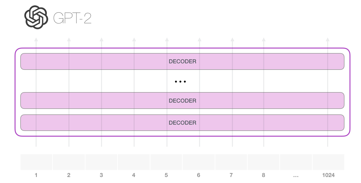
An LLM is the decoder half of the 2017 Transformer, stacked deep, with one structural tweak: causal masking. The training objective is deceptively simple: predict the next token. That alone, at internet scale, produces a model that implicitly knows grammar, facts, and a surprising amount of reasoning.
But raw pretraining gets you a text completer and stops short of an assistant. Supervised fine-tuning (SFT) teaches it to answer in the right format. Preference optimization (RLHF or DPO) teaches it which of several plausible answers humans prefer. One sentence for an interview: an LLM is next-token prediction, scaled up and then aligned.
01Intuition
An LLM is not a new architecture. It's the decoder half of the transformer you already know, with nothing else attached.
In 08 you met two flavors of transformer block:
- Encoder block. Bidirectional. Every token sees every other token in both directions. The BERT half.
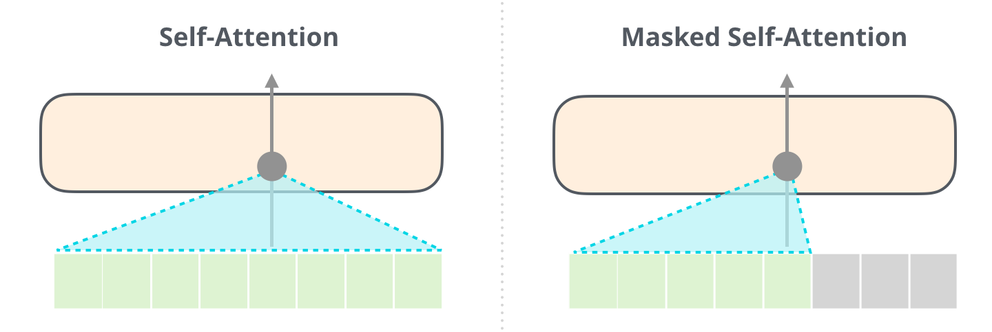
- Decoder block. Causal. A token sees only itself and whatever came before it.
Turning that into "an LLM" in the GPT/decoder-only sense takes one structural change:
- Keep only the causal block.
- Stack it 12 to 100+ times.
- Put a vocabulary-sized output layer on top.
Nothing new is needed: no new attention mechanism and no new normalization trick. Delete the encoder and cross-attention, and stack the piece you already understand.
The training objective is almost insultingly simple. Given some text, predict the next token. Given "The capital of France is", predict "Paris".
This is next-token prediction. It works so well because it is free supervision: every sentence ever written is automatically a training example, and no human needs to label anything.
To get good at next-token prediction across a large and diverse enough pile of text, the model is forced to implicitly learn much more than "what word comes next."
- Predicting the token after "The capital of France is" requires encoding the fact that Paris is that capital.
- Predicting the next line of a step-by-step derivation requires tracking the intermediate state of the problem, and mimicking surface style is not enough.
- Predicting the next token in grammatical text requires an implicit model of syntax.
None of this is programmed in. It falls out as a side effect of being good at the one task the model was asked to do.
What next-token prediction alone does not give you is a model that behaves like an assistant. Left alone, a pretrained model just continues text plausibly. Asked a question, it might answer. It might restate the question. It might trail off into a list of similar questions. All of those follow a question somewhere on the internet.
Getting from "plausible continuation of internet text" to "helpful, on-format answer that stops in the right place" is the job of everything after pretraining: SFT, then RLHF or DPO, which is most of the rest of this page.
A language model predicts the next word. The simplest possible one just counts what followed each word in its training text.
Try it Learn which word follows which from ten words of text
from collections import Counter, defaultdict

text = "the cat sat on the mat and the cat ran".split()
nxt = defaultdict(Counter)
for a, b in zip(text, text[1:]):
    nxt[a][b] += 1                      # count what follows each word

for word in ("the", "cat"):
    total = sum(nxt[word].values())
    probs = {w: round(c / total, 2) for w, c in nxt[word].items()}
print(f"after '{word}':", probs)the, this model gives cat two chances in three and mat one in three. In the text, the was followed by cat twice and mat once. After cat it splits evenly between sat and ran. A large language model does the same job, giving a probability to every possible next token, with far more context and a learned function in place of a lookup table.02Timeline
Each NLP task had its own architecture, or at least its own fine-tuned copy with a separate head, even after pretrained embeddings and BERT-style fine-tuning.
GPT (2018) showed one decoder-only transformer pretrained on next-token prediction could beat task-specific models, and GPT-3 (2020, 175B parameters) needed no fine-tuning for many tasks, only a few examples in the prompt.
In 2022, InstructGPT showed that SFT followed by RLHF turns a pretrained completer into an instruction-follower, and Chinchilla showed most large models were undertrained for their size, which changed how labs split compute between model size and data.
03Architecture: from decoder-only block to training pipeline
The one structural change from 08: causal masking
Take the exact block-anatomy diagram from 08 (LayerNorm, multi-head self-attention, residual add, LayerNorm, feed-forward, residual add) and relabel it almost unchanged. The only thing that turns it into a GPT-style block is masking. Before the softmax in $QK^\top$, every score for a key position after the query position gets set to $-\infty$. So position $i$ can only attend to positions $\le i$.
Stack that block $N$ times, add a final LayerNorm and a linear projection from $d_{model}$ back to vocabulary size, and you have a decoder-only LLM.
Tokenization: why vocabulary size is a real design tradeoff
An LLM doesn't read characters or whole words. It reads tokens: chunks produced by a subword tokenizer, almost always something in the BPE (byte-pair encoding) family. Conceptually, start from individual characters or bytes, then repeatedly merge the most frequent adjacent pair into a new token.
The result is a vocabulary that mixes common whole words ("the" ends up as one token) with subword pieces for anything rarer. Any string can still be represented, because you can always fall back to individual characters or bytes. There's no "unknown token" escape hatch the way there was for whole-word vocabularies.
Vocabulary size is a genuine three-way tradeoff and no free parameter to crank up.
- Bigger vocabulary packs more meaning per token. The same text becomes a shorter sequence, so less compute is spent per unit of content, since attention cost grows with sequence length (08).
- But bigger costs you twice. A larger embedding table and output projection (both scale with vocab size $\times\ d_{model}$), and rarer tokens see less training signal each, since the same corpus spreads its counts across more distinct ids.
- Smaller vocabulary keeps those tables lean and gives every token plenty of signal. But it burns more context budget on ordinary text, and shreds rare words (a chemical name, a low-resource language) into many small pieces just to represent them.
Embedding table, output projection, and weight tying
The embedding table maps each of the $V$ vocabulary ids to a learned $d_{model}$-dimensional vector: a $(V, d_{model})$ lookup table, trained like any other weight. The output projection does the mirror-image job. It maps the final hidden state back to a $V$-dimensional vector of logits, which softmax turns into the next-token distribution.
Both matrices are the same shape transposed, so it's common to share the weights between them, which is weight tying. It cuts a real chunk of parameters (these tables can be a large fraction of total parameters in smaller models) and tends to regularize training, since the same vector now has to work both as "what this token means going in" and "what this token would mean coming out."
The training pipeline, end to end
Pretraining alone gives you a next-token predictor with broad implicit knowledge and no idea how to behave like an assistant. Getting from there to a usable model takes a pipeline of steps:
Scaling laws: Chinchilla and the size/data tradeoff
Training compute is well approximated by $C \approx 6ND$ FLOPs, where $N$ is parameter count and $D$ is training tokens (roughly 2 FLOPs per parameter per token forward, another 4 backward).
Before 2022, the implicit assumption behind most large-model training was "bigger model, better model": pour a fixed budget mostly into $N$ and train on whatever $D$ happens to fit the schedule. Hoffmann et al.'s Chinchilla paper (2022) tested that directly, training over 400 models across a range of sizes and token counts and fitting how loss depends on both under a fixed compute budget.
Their finding: loss is minimized when $N$ and $D$ scale together, roughly proportionally. That works out to about 20 training tokens per parameter in their fitted regime, and maximizing $N$ alone is not the answer. Fix $C$ and this becomes a genuine tradeoff. Spend the budget on a bigger model and $D$ must shrink. Spend it on more data and $N$ must shrink.
Chinchilla itself was 70B parameters trained on roughly 4x more tokens than Gopher (280B parameters) for the same training compute. It beat Gopher, GPT-3, and other larger contemporaries trained on that older, size-heavy recipe. The practical consequence: model size and data budget aren't separable choices you pick in isolation. A model that is "big enough" but starved of tokens for its size is, in Chinchilla's own framing, substantially undertrained.
Supervised fine-tuning (SFT)
A freshly pretrained model is a very good predictor of "whatever plausibly follows this text." That includes answering your question. It also includes restating it, imitating a bad forum reply, or trailing off, because all of those are plausible continuations of internet text too.
SFT fixes this with the exact same next-token-prediction loss you already know, on a different and much smaller curated dataset: (instruction, ideal response) pairs, usually written or vetted by humans, in a consistent template. The model is trained to predict the response tokens given the instruction. No new architecture, no new loss. Just a distribution shift in what "plausible continuation" means.
This step alone turns a raw completer into something that reliably answers in the right format and stops in the right place. The alignment stages that follow refine which of several plausible SFT-style answers humans prefer. They don't teach instruction-following from scratch.
Preference optimization: RLHF vs DPO
SFT teaches a plausible, on-format response. It doesn't teach the model which of several plausible responses people prefer: more concise vs. more thorough, direct vs. hedged, correct-but-blunt vs. correct-and-tactful. That is a preference and not a fact you can supervise with one correct label, which is what the stage after SFT is for.
Two recipes dominate:
- RLHF, used for InstructGPT (2022). Train a separate reward model on human-labeled comparisons ("given two responses to this prompt, which do you prefer?"). Then run an actual reinforcement-learning loop (PPO) that updates the SFT model toward higher-reward outputs, with a KL penalty holding it close to the SFT starting point so it doesn't drift into degenerate, reward-hacking territory.
- DPO (2023). Reaches the same alignment objective through a mathematical shortcut, spelled out term by term in the Math section below. It skips the reward model and the RL loop and optimizes directly on the preference pairs with a single supervised-style loss.
Quantization and LoRA/QLoRA: the two big levers for cheap adaptation and deployment
These solve two different problems that get conflated because they are often used together.
Quantization is a deployment lever: take an already-trained model's weights, stored in 16-bit floating point, and represent them with fewer bits: 8-bit, 4-bit, sometimes lower. That shrinks memory footprint and often speeds up inference, at the cost of some numerical precision. Two variants:
- Post-training quantization (PTQ). Done after training with no gradient updates, just a calibration pass to pick good quantization ranges. Cheap, with usually small but non-uniform quality loss (arithmetic and rare factual recall tend to degrade first).
- Quantization-aware training (QAT). Simulates the quantization during training, so the weights adapt to the precision loss as they are learned. Better accuracy at the target precision, at the cost of an actual training run.
LoRA is an adaptation lever, not a deployment one. Instead of updating all of a pretrained model's weights during fine-tuning, freeze the base weight matrix $W_0$ entirely and learn a small low-rank update alongside it: $W = W_0 + BA$, where $B \in \mathbb{R}^{d\times r}$, $A \in \mathbb{R}^{r\times k}$, and the rank $r$ is tiny compared to $d$ and $k$.
You back-propagate into only $B$ and $A$, a tiny fraction of the parameter count. That drastically cuts optimizer memory and lets you store and swap many task-specific adapters against one shared frozen base.
QLoRA combines both levers: quantize the frozen base to 4-bit to shrink memory further, then run LoRA fine-tuning on top of that quantized base. This is what makes fine-tuning a large model feasible on a single consumer-class GPU.
Mixture-of-experts: decoupling parameter count from compute-per-token
A dense transformer's feed-forward layer runs every token through the same weights. More parameters there means more compute for every token without exception. MoE breaks that coupling. Replace the single FFN with a bank of $E$ parallel expert FFNs plus a small learned router. For each token, the router selects only the top-$k$ experts (commonly 1 or 2) to run.
Here $g_i(x)$ is the router's weight for expert $i$ on input $x$. Only the selected experts do any compute; the rest cost nothing for that token. The result: a model can have an enormous total parameter count spread across all its experts, while compute per forward pass reflects only the handful activated. More total capacity, without paying its full compute cost on every token.
The cost shows up in training. Without an auxiliary load-balancing loss encouraging the router to spread tokens evenly, it collapses onto a favorite few experts, and you lose the benefit you paid to build.
Serving basics
Two things matter at a conceptual level, because they shape how you reason about training and architecture choices:
- The KV cache (introduced in 08). During autoregressive generation the model caches every past token's key and value vectors instead of recomputing attention over the whole prefix at every step. It is now a first-class cost of running an LLM product, often the dominant memory consumer on a serving GPU for long conversations.
- Batching. A serving system groups multiple requests together so the GPU processes them in parallel, trading a little per-request latency for much higher throughput.
The deep systems treatment (paged attention, continuous batching, tensor/pipeline parallelism, and quantization-for-serving tradeoffs) lives in 23 (Efficient AI & Systems). This page covers only what you need to reason about training and architecture tradeoffs, and leaves out how to operate a serving fleet.
The long tail, briefly
- Data quality, dedup, and mixture design. A pretraining corpus isn't just "all the text you can find." Near-duplicate documents inflate a dataset without adding signal and push the model toward memorizing repeated substrings — deduplication is a standard pipeline step because it measurably improves quality per token spent. Mixture design — what fraction of tokens come from web text vs. books vs. code vs. curated sources — meaningfully shapes what the model is good at; a heavier code mixture improves structured reasoning, not by accident but because code text rewards tracking state precisely.
- Long-context training. A model pretrained mostly on short documents doesn't automatically use a 128k-token window well just because attention can mathematically handle it (see 08 on attention sinks and mid-context dilution) — labs run dedicated long-context stages, often extending position embeddings and training on long documents, specifically to make the model exploit long context rather than merely tolerate it.
- Function/tool calling. A trained (or prompted) behavior where the model emits a structured request — "call this API with these arguments" — instead of answering purely from its own weights, then consumes the tool's result before producing a final answer. This is what turns a text predictor into something that can look things up, run code, or take actions, and it's the entire foundation of 11 (RAG & agents).
- Structured/constrained decoding. An inference-time technique, not a training change: instead of hoping free-form output happens to be valid JSON, constrain token-by-token sampling itself so only tokens consistent with a target grammar are ever eligible — a decoding-time guarantee that output can't be unparseable, no retraining required.
- Code, multilingual, and domain models. Code models are typically the same decoder-only architecture, pretrained or fine-tuned with a much heavier proportion of source code, often trained to fill in the middle of a file rather than only continue it left-to-right. Multilingual and domain models face the tokenization tradeoff most acutely — a tokenizer trained mostly on English badly over-fragments other languages or specialized vocabularies (legal text, chemistry), quietly costing context budget and quality unless the tokenizer and pretraining mixture are built for that domain from the start.
- Distillation, pruning, and model merging. Distillation trains a smaller student model to match a larger teacher's output distribution — a genuine training run, but it typically preserves more capability per parameter than quantizing the teacher down to the same footprint. Merging averages or interpolates the weights of multiple fine-tuned variants of the same base model directly, no training required, and works surprisingly often when the variants stayed close to the same base. Pruning removes weights or structures judged least important, usually followed by a short fine-tune to recover quality — the least reliably clean win of the three for modern LLMs.
04The equations
Next-token prediction loss
- x₁...x_T the training sequence — the same tokens serve as both input and, one position later, label. No separate annotation exists or is needed.
- P_θ(x_t | x<t) the probability the model assigns to the actual next token, read straight off the softmax over vocabulary-sized logits at position $t-1$.
- Σ over t the causal mask lets every position's prediction be computed in one parallel forward pass (teacher forcing) — one sequence of length $T$ yields $T$ training signals for free.
- minimize L equivalent to maximizing the likelihood the model assigns to the real continuation of text it was trained on — nothing more exotic than that is happening during pretraining.
DPO loss
- x, y_w, y_l a prompt $x$ with a human-labeled preference pair: $y_w$ the preferred ("winning") response, $y_l$ the dispreferred ("losing") one.
- π_θ, π_ref $\pi_\theta$ is the policy being trained; $\pi_{\text{ref}}$ is a frozen reference model, almost always the SFT checkpoint before preference tuning starts.
- log ratio how much more (or less) likely the current model makes a response compared to where it started — the quantity being pushed around, not a raw probability.
- β controls how hard to push. Higher $\beta$ trusts the preference data more and allows a bigger departure from $\pi_{\text{ref}}$; lower $\beta$ keeps the model closer to its starting point — it plays the same role the KL penalty plays in RLHF.
- σ turns the gap between "how much the winning response's relative likelihood moved up" and "how much the losing response's moved up" into a probability that this pair is correctly ordered — the loss is binary cross-entropy on that probability against "yes, correctly ordered."
- net effect push up the relative likelihood of preferred responses and down the relative likelihood of dispreferred ones, with no separate reward model and no RL rollout loop — the reward is implicit in the likelihood ratio itself, which is the "secretly a reward model" of the paper's title.
05Why these choices
Why decoder-only won over encoder-decoder for general-purpose LLMs
Encoder-decoder makes sense when input and output are structurally different sequences with a clean split: a source sentence and a target sentence in translation, a document and its summary.
A general-purpose assistant has no such split. The "task" might be a question, a document to summarize, code to complete, or a partial conversation. The boundary between prompt and completion is just wherever generation happens to start, not a structural property baked into the task.
Decoder-only treats the prompt as a prefix in the same sequence as the completion, processed by the exact same weights and the exact same causal-attention mechanism as the response. There is no architectural commitment to a fixed input/output split, so one model handles completion, question-answering, chat, and code without changing shape.
It also composes naturally with in-context learning. The whole context (instructions, examples, new query) is one sequence attended to causally, so the model reads a few examples immediately before generating. This is what GPT-3's few-shot prompting exploits.
Why DPO gained adoption alongside — and often instead of — full RLHF
Standard RLHF needs three models trained in sequence: the SFT model, a reward model trained on human preference pairs, and a policy optimized against that reward model with PPO. That last stage is a genuine RL loop, with rollouts, a value function, clipping, and the usual RL instability and reward-hacking risk.
The optimal policy for that same KL-constrained RLHF objective has a closed form directly in terms of the reward function.
Substitute that closed form into the Bradley-Terry preference model already used to train the reward model, and the reward model cancels out algebraically. What is left is a loss defined purely on the policy's own likelihoods for preferred vs. dispreferred responses.
DPO reaches the same alignment objective in theory with one supervised-style training loop instead of three sequential stages, with no reward model to maintain separately and no PPO rollouts. That is why DPO and its descendants spread quickly through open-source and production fine-tuning pipelines after 2023.
06Complexity, failure modes, and what breaks
| RLHF (PPO) | DPO | |
|---|---|---|
| Training complexity | 3 stages: SFT, reward model, PPO policy optimization | 2 stages: SFT, then a direct preference loss |
| Stability | Genuine RL training — sensitive to hyperparameters, can diverge or reward-hack | Supervised-style loss — generally more stable to train |
| What you need | A separate reward model plus RL infrastructure: rollouts, value function, PPO clipping | Just the preference-pair dataset and a frozen reference copy of the SFT model |
| Typical use | Frontier labs with engineering budget for more explicit control over the reward signal | Default choice for most open-source and production fine-tuning pipelines |
What shows up in production
- Reward hacking. The policy finds outputs that score well on an imperfect reward model or preference signal without being better — longer answers, hedging language, sycophantic agreement — because those correlate with human preference ratings, even though they aren't more correct.
- Overfitting to a narrow preference-annotator population. Preference data reflects the taste, culture, and instructions given to whichever annotator pool labeled it. The aligned model inherits those biases as if they were universal — "helpfulness" quietly comes to mean "what this specific annotator pool liked."
- Quantization accuracy loss. Lower precision trades a usually small, but non-uniform, amount of task accuracy for large memory and compute savings — arithmetic and low-frequency facts tend to degrade before fluent generation does.
- MoE load-balancing issues. An unregularized router collapses onto a favorite handful of experts, wasting the extra capacity and effectively shrinking the model back toward its active-parameter count — the reason MoE training adds an auxiliary load-balancing loss term.
Reasoning-focused post-training is an active, fast-moving research area: extra RL or search-based training aimed specifically at multi-step problem solving, layered on top of the SFT/RLHF/DPO recipe described here. So are preference-optimization variants that go beyond vanilla DPO.
Treat the exact recipe used by any specific current model as a moving target. The underlying building blocks (pretraining, SFT, preference optimization, quantized deployment) are stable enough to learn thoroughly, whichever variant is fashionable this quarter.
07Build this
A scaling law reads like a claim about somebody else's compute budget. Three small training runs on your own laptop turn it into a line you drew yourself.
Train the same decoder-only model at three sizes on one small corpus, then plot final validation loss against parameter count on log axes. The task is ordinary next-token prediction, and the samples are not the interesting part. The shape of the three points is, because that shape is section 03's scaling argument drawn from runs you can afford.
- Take a few megabytes of plain text. Anything with consistent style works: one book, one codebase, one set of transcripts. Hold out a slice for validation.
- Train a BPE tokenizer on that corpus with a small vocabulary, a few thousand merges. Print the merge list in order and read the first hundred. Watch characters assemble into common suffixes, then into whole words.
- Build the decoder block by hand from the diagram in section 03: LayerNorm, masked self-attention, residual add, LayerNorm, feed-forward, residual add. Write the causal mask yourself with
torch.tril. Nonn.TransformerDecoder. - Train three models that differ by roughly an order of magnitude in parameter count each, varying width and depth. Same data, same number of tokens seen, same optimizer, same schedule. Only size changes.
- Plot final validation loss against parameter count with both axes log-scaled. Sample a paragraph from each model and read them side by side.
- Now break it deliberately. Delete the causal mask from the smallest model and retrain.
Where this runs in production
A modern assistant product's pipeline maps onto this page almost exactly:
- Pretraining. Web-scale next-token prediction builds the base model's broad knowledge and language competence.
- SFT. Curated instruction-response pairs teach it to answer on-format.
- Preference optimization. RLHF or DPO, using human or model-assisted preference judgments, teaches it which of several plausible answers people want.
- Deployment. The resulting weights are quantized, and sometimes distilled into a smaller model, to make serving affordable, with KV-cache and batching handling request-level efficiency (full treatment in 23).
Everything sitting on top at inference time (a system prompt, tool/function-calling scaffolding, retrieval) is applied to this already-trained stack and is not baked into training. That is where 11 picks up.
08Interview questions
BeginnerWhat's the actual training signal used to pretrain an LLM, and where do the "labels" come from?
Every token in a training sequence is simultaneously an input (for predicting later tokens) and a label (the correct answer for predicting it, given everything before it). Teacher forcing exploits this directly: feed the model the true previous tokens, ask it to predict the next one, compute cross-entropy against the actual next token, and repeat for every position in the sequence in parallel via the causal mask. No human labels this data — the label is just "whatever token comes next in text that already existed" — which is why pretraining can use effectively the entire scrapeable internet as its own supervision.
BeginnerWhat's the one structural difference between the encoder blocks in 08 (BERT) and the blocks used in a GPT-style LLM?
Causal masking. A decoder-only block adds a mask before the softmax that sets the score for any key position after the query position to $-\infty$, so a token's attention output can only depend on tokens at or before it. An encoder block has no such mask — every token attends to every other token, forward and backward. Everything else — Q/K/V projections, multi-head split, residual connections, LayerNorm, the feed-forward layer — is identical.
IntermediateExplain the difference between RLHF and DPO.
RLHF trains a separate reward model on human preference pairs, then runs PPO — an actual RL loop with rollouts, a value function, and clipping — to optimize the policy against that learned reward, with a KL penalty holding it near the SFT model. DPO skips both the reward model and the RL loop: it shows the optimal policy for that same KL-constrained objective has a closed form in terms of log-probability ratios between the trained policy and a frozen reference policy, so preference pairs can be optimized directly with one supervised-style loss. Same underlying alignment objective, reached with far less machinery and instability — at the cost of somewhat less explicit control over the reward signal.
IntermediateWhy would you reach for LoRA instead of full fine-tuning?
LoRA freezes the entire pretrained weight matrix and learns a small low-rank update, $W=W_0+BA$, updating only $B$ and $A$ — orders of magnitude fewer parameters than the full model. That means far less optimizer state in memory, a much smaller checkpoint per fine-tuned task, and the ability to swap adapters in and out of one shared frozen base at serving time. Full fine-tuning still wins on raw quality ceiling when you have the compute and data to justify it; LoRA (and QLoRA, which additionally quantizes the frozen base to 4-bit) is about making adaptation cheap, not about beating full fine-tuning outright.
IntermediateWhat does a mixture-of-experts layer change about the forward pass compared to a dense FFN?
A dense FFN runs every token through the same weights, so more parameters means more compute per token, always. An MoE layer replaces the single FFN with many parallel expert FFNs plus a router that picks the top-k experts (often 1 or 2) per token — only those experts do any compute for that token. This decouples total parameter count from compute-per-token: the model can have a huge total parameter count spread across experts while any single forward pass only touches a small fraction of them. The catch is the router — without a load-balancing loss it collapses onto a favorite few experts and the extra capacity goes to waste.
DeepWhy do Chinchilla-style scaling laws matter for a training budget decision?
Because compute is the actual constraint, and Chinchilla showed loss is minimized under a fixed compute budget by scaling model size and training tokens together — roughly 20 tokens per parameter in their fitted regime — not by maximizing parameters and undertraining on whatever data fits. Pick a model twice as large as compute-optimal for your budget and you're forced to train it on fewer tokens than compute-optimal, ending up worse than a smaller model trained longer on the same budget — which is exactly what several pre-2022 large models did, by Chinchilla's own comparisons. Practically: the model-size decision and the data-budget decision aren't separable — you size the model to the compute and quality data you actually have.
DeepYou need a 70B-quality model to run in a 15B-model's memory footprint. What are your options, and what does each cost you?
Quantization: compress the same weights to lower precision, cutting memory roughly 2–4x with typically small but non-uniform accuracy loss. Distillation: train a genuinely smaller model to mimic the larger model's output distribution — a real training run, but it usually preserves more capability per parameter than quantization alone. Pruning: remove weights or structures judged least important, then fine-tune to recover quality — the least reliably clean win of the three for modern LLMs. Or start over: per Chinchilla, a smaller model trained compute-optimally can beat an undertrained larger one at the same budget. In practice: quantize first since it's the cheapest and most reliable win, layer in distillation or a purpose-trained smaller model if that's not enough, and benchmark on your actual task, since accuracy loss from any of these is rarely uniform across tasks.
DeepWhy can pushing a preference-optimization objective too hard make a model worse, even though the reward or preference signal keeps improving?
The reward model (RLHF) or the implicit preference signal (DPO) is a proxy for what humans actually want, not the thing itself — and proxies can be gamed. Optimize too aggressively against a reward model, or let DPO's $\beta$ get too permissive relative to the reference model, and the policy finds outputs that score well on the proxy — longer answers, hedging, sycophantic agreement — without those outputs being more correct or useful. That's reward hacking, and it's exactly why RLHF keeps a KL penalty (and DPO's $\beta$ plays the same role) tethering the policy back to the reference model. Weaken that tether and gains on the training signal can actively diverge from real quality.
09Go deeper
●Now write it yourself
Reading the derivation and being able to produce it are different skills. These are Deep-ML problems that exercise what this page covers — each one is checked against real test cases, not multiple choice.
Matched to this page from Deep-ML's catalogue of 1,380 problems. More at deep-ml.com, and Where to practise covers the other platforms and what each one trains.